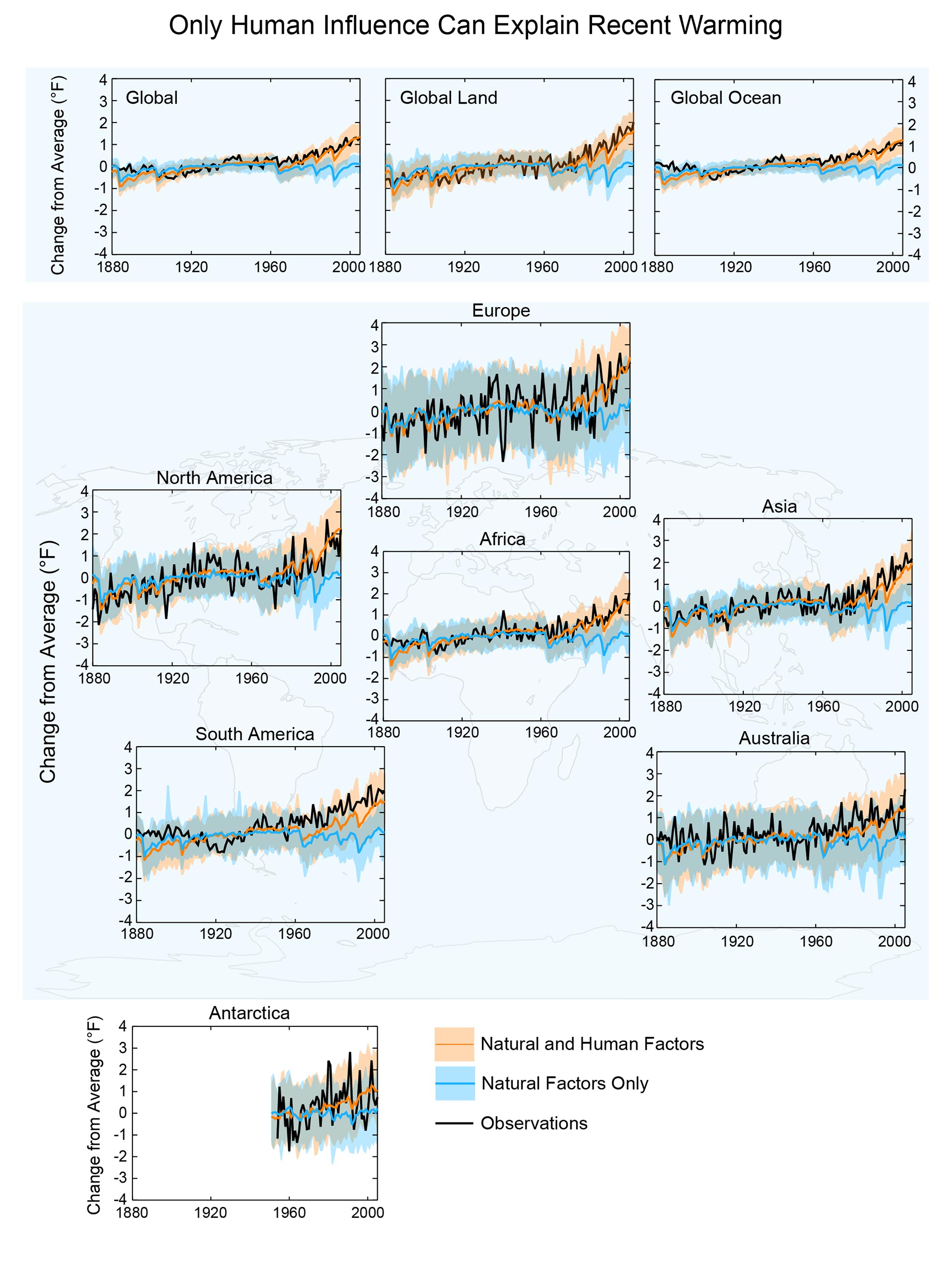
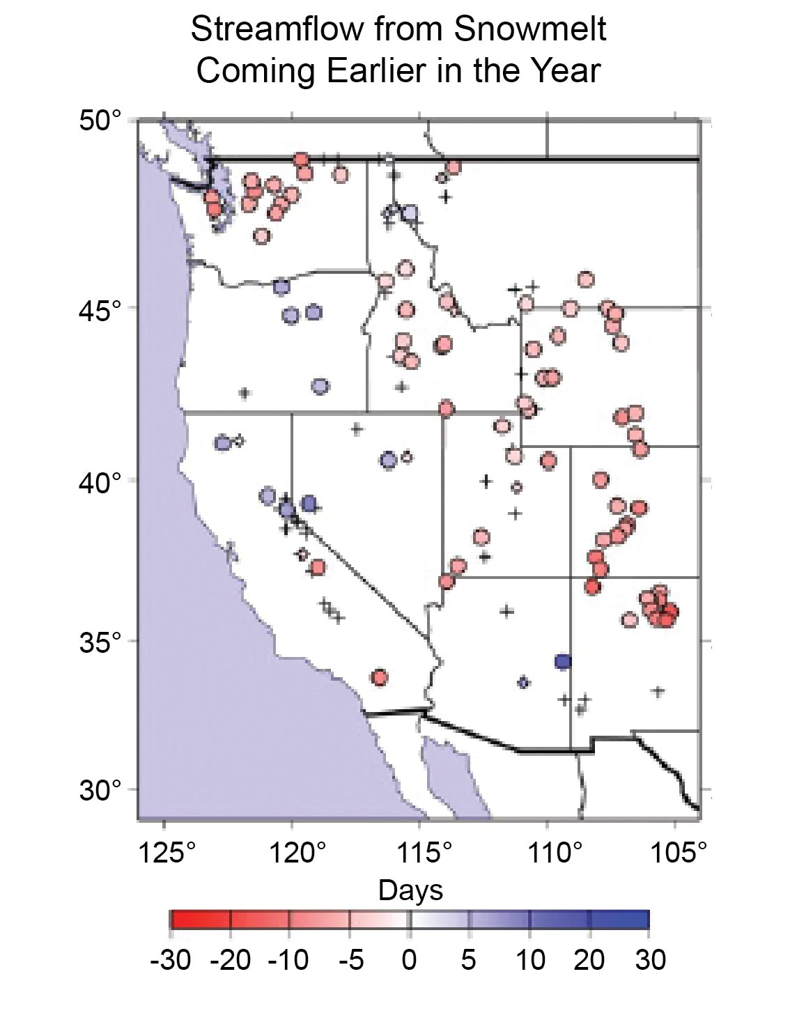
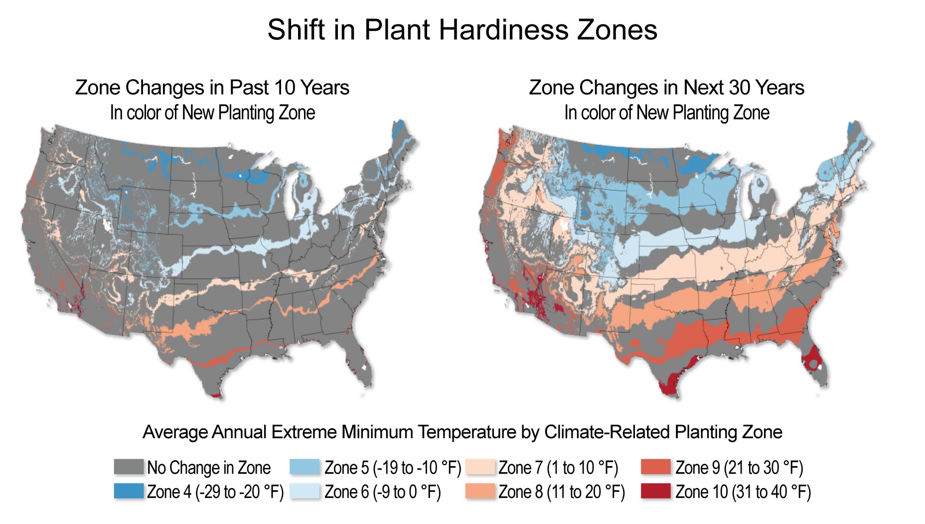
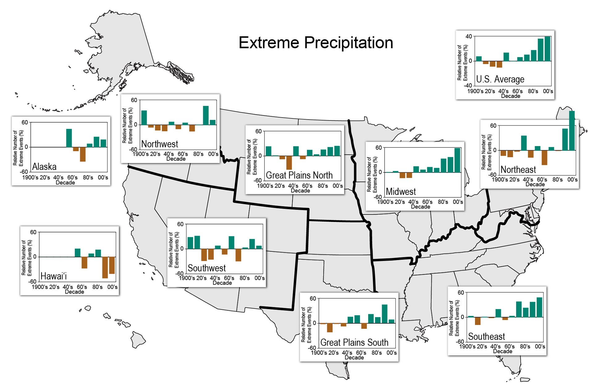
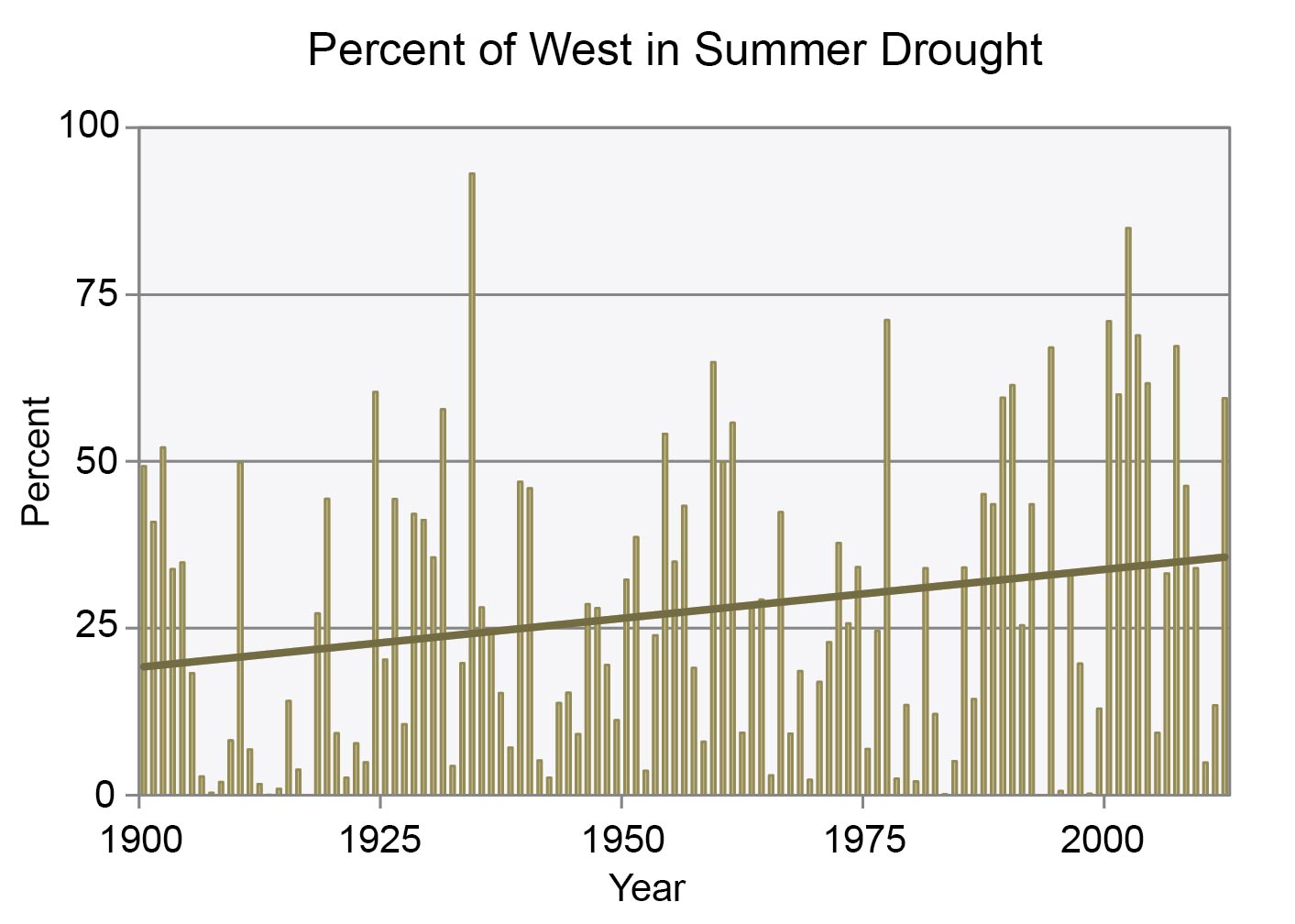
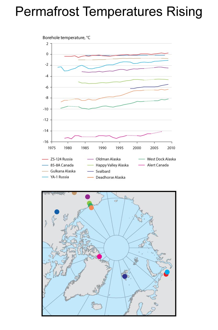
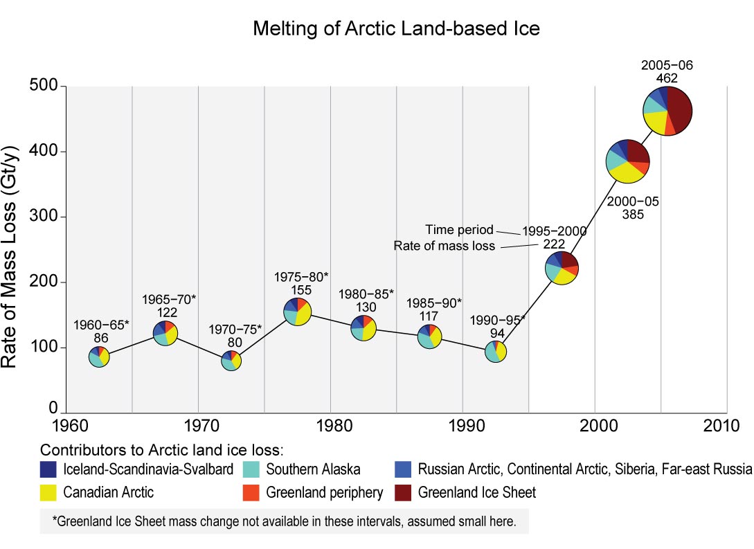
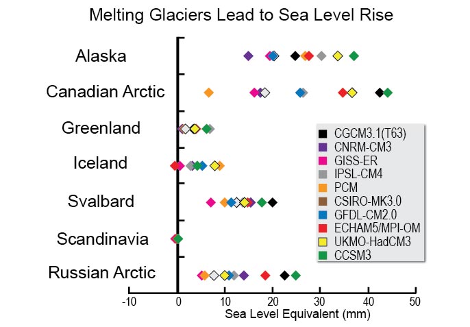
This website is the digital version of the 2014 National Climate Assessment, produced in collaboration with the U.S. Global Change Research Program.

For the official version, please refer to the PDF in the downloads section. The downloadable PDF is the official version of the 2014 National Climate Assessment.

Credits | Site Map

Search Options

X

Search form

Top

Welcome to the National Climate Assessment

The National Climate Assessment summarizes the impacts of climate change on the United States, now and in the future.

A team of more than 300 experts guided by a 60-member Federal Advisory Committee produced the report, which was extensively reviewed by the public and experts, including federal agencies and a panel of the National Academy of Sciences.

Explore the effects of climate change
United States Global Change Research Program logo
United States Department of Agriculture logo United States Department of Commerce logo United States Department of Defense logo United States Department of Energy logo United States Department of Health and Human Services logo United States Department of the Interior logo United States Department of State logo United States Department of Transportation logo United States Environmental Protection Agency logo National Aeronautics and Space Administration logo National Science Foundation logo Smithsonian Institution logo United States Agency for International Development logo

Climate Science Supplement

This appendix provides additional information about climate science. It expands on the Our Changing Climate section by providing more details on what is happening to climate, how we know that these changes are mainly due to human activities, and what changes are projected for the future.

Next

Convening Lead Authors

John Walsh, University of Alaska Fairbanks

Donald Wuebbles, University of Illinois

Lead Authors

Katharine Hayhoe, Texas Tech University

James Kossin, NOAA, National Climatic Data Center

Kenneth Kunkel, CICS-NC, North Carolina State Univ., NOAA National Climatic Data Center

Graeme Stephens, NASA Jet Propulsion Laboratory

Peter Thorne, Nansen Environmental and Remote Sensing Center

Russell Vose, NOAA National Climatic Data Center

Michael Wehner, Lawrence Berkeley National Laboratory

Josh Willis, NASA Jet Propulsion Laboratory

Contributing Authors

David Anderson, NOAA, National Climatic Data Center

Viatcheslav Kharin, Canadian Centre for Climate Modelling and Analysis, Environment Canada

Thomas Knutson, NOAA Geophysical Fluid Dynamics Laboratory

Felix Landerer, NASA Jet Propulsion Laboratory

Tim Lenton, Exeter University

Richard Somerville, Scripps Institution of Oceanography, Univ. of California, San Diego

Introduction

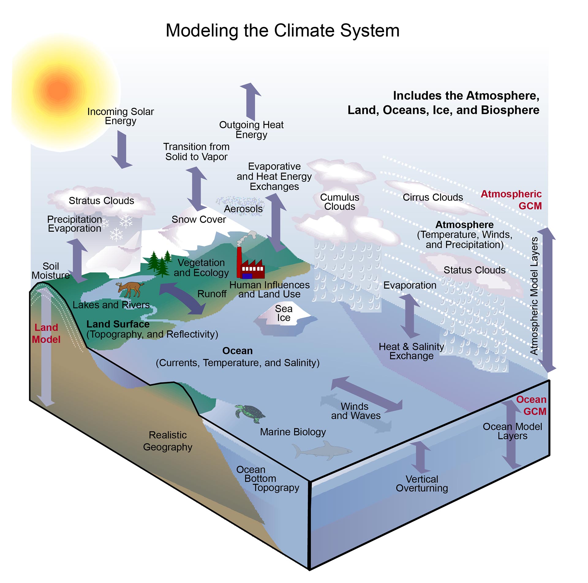
This appendix provides further information and discussion on climate science beyond that presented in Ch. 2: Our Changing Climate. Like the chapter, the appendix focuses on the observations, model simulations, and other analyses that explain what is happening to climate at the national and global scales, why these changes are occurring, and how climate is projected to change throughout this century. In the appendix, however, more information is provided on attribution, spatial and temporal detail, and physical mechanisms than could be covered within the length constraints of the main chapter.

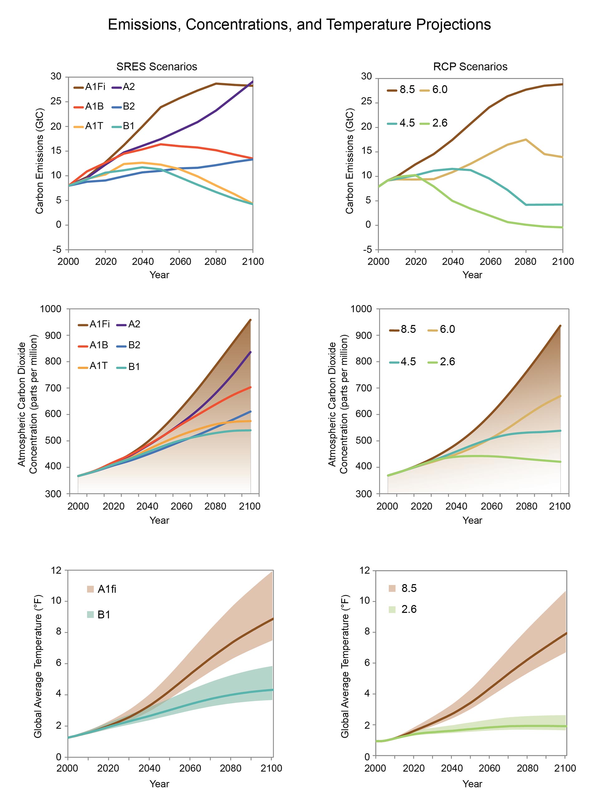
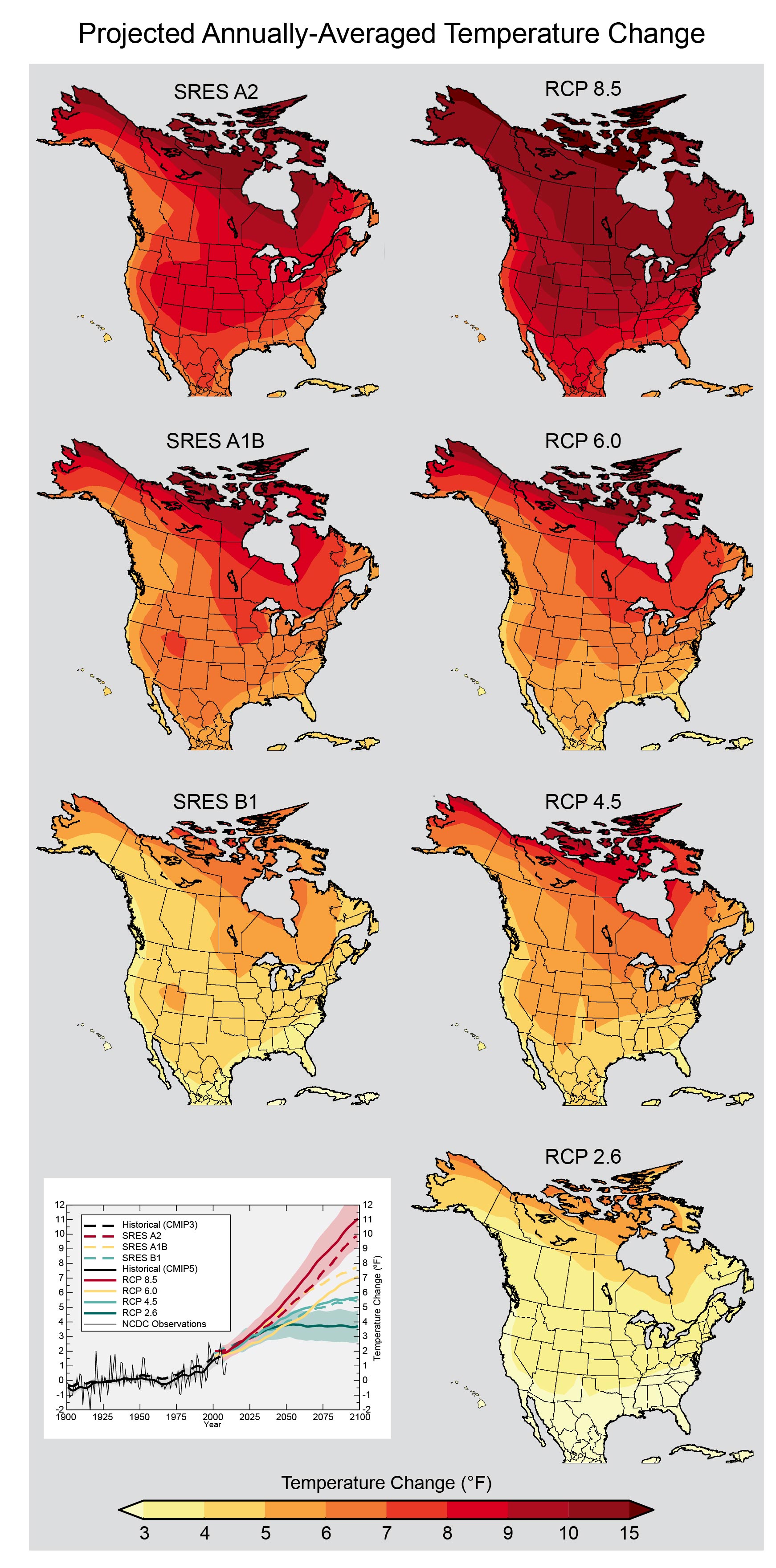
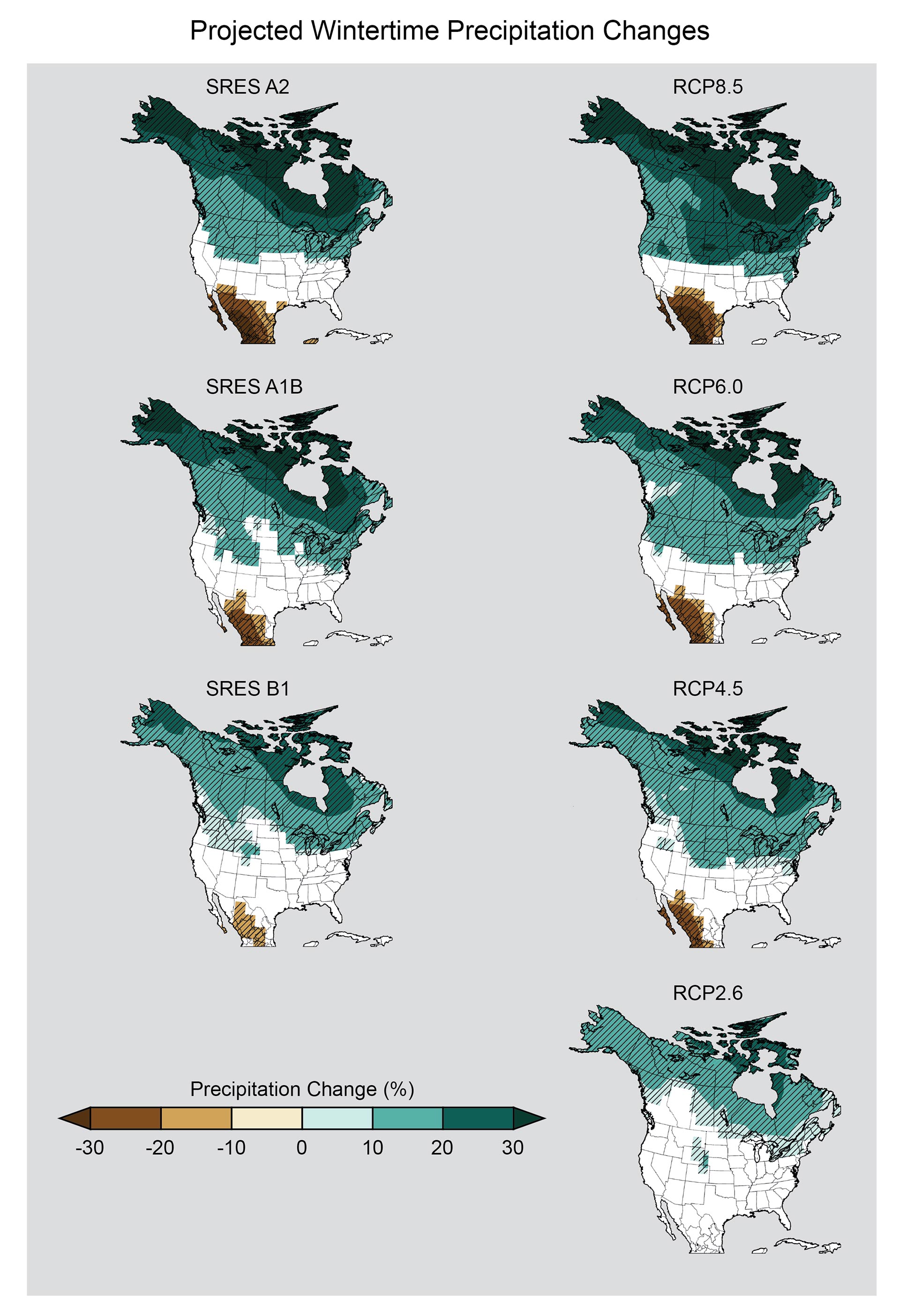
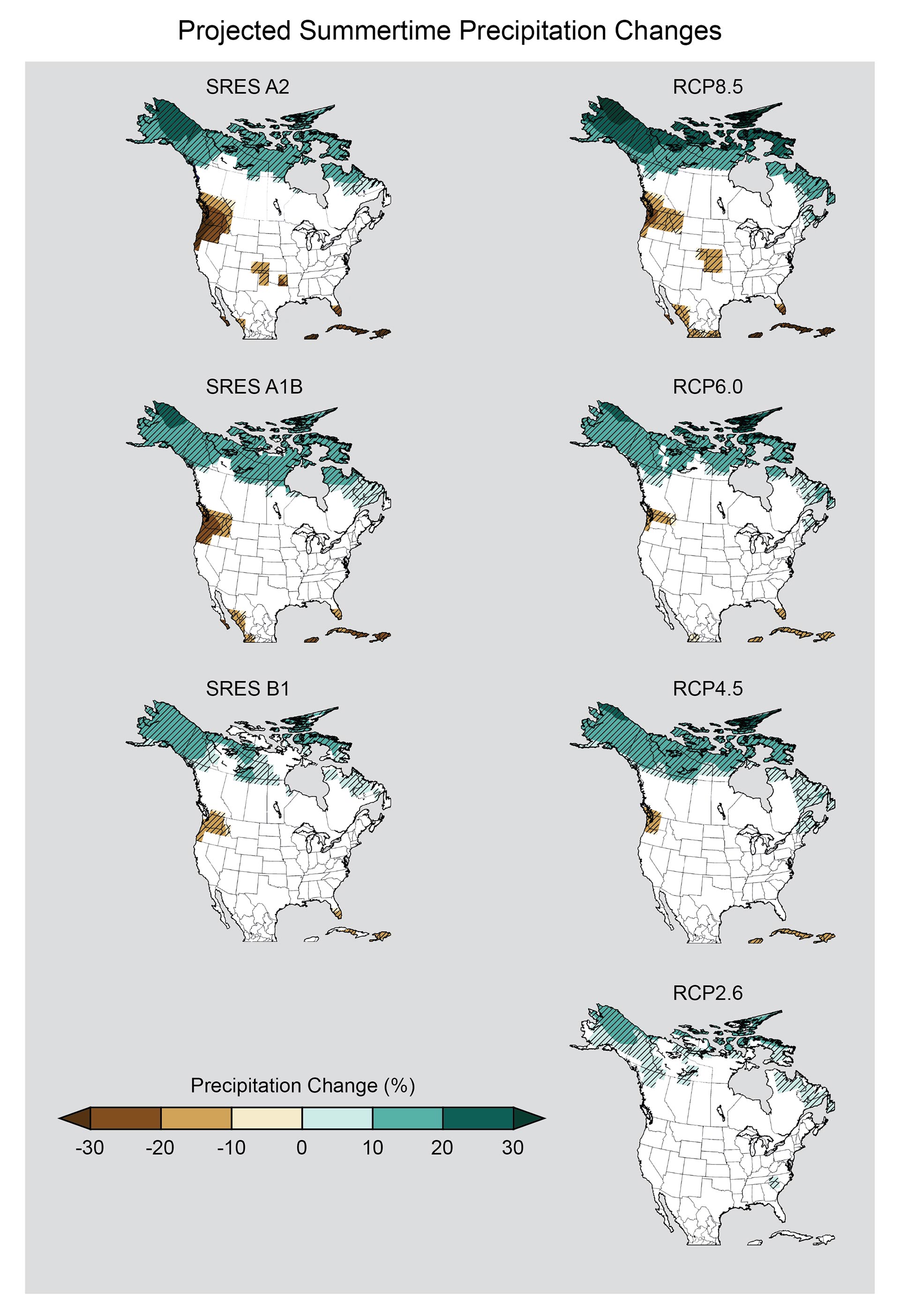
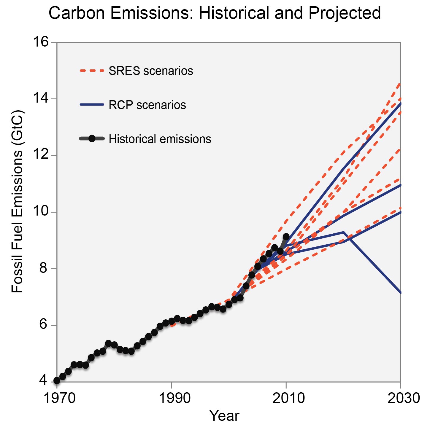
As noted in the main chapter, changes in climate, and the nature and causes of these changes, have been comprehensively discussed in a number of other reports, including the 2009 assessment: Global Climate Change Impacts in the United States139 and the global assessments produced by the Intergovernmental Panel on Climate Change (IPCC) and the U.S. National Academy of Sciences. This appendix provides an updated discussion of global change in the first few supplemental messages, followed by messages focusing on the changes having the greatest impacts (and potential impacts) on the United States. The projections described in this appendix are based, to the extent possible, on the CMIP5 model simulations. However, given the timing of this report relative to the evolution of the CMIP5 archive, some projections are necessarily based on CMIP3 simulations. (See Supplemental Message 5 for more on these simulations and related future scenarios).

Supplemental Message 1

Although climate changes in the past have been caused by natural factors, human activities are now the dominant agents of change. Human activities are affecting climate through increasing atmospheric levels of heat-trapping gases and other substances, including particles.

Supplemental Message 1

The Earth’s climate has long been known to change in response to natural external forcings. These include variations in the energy received from the sun, volcanic eruptions, and changes in the Earth’s orbit, which affects the distribution of sunlight across the world. The Earth’s climate is also affected by factors that are internal to the climate system, which are the result of complex interactions between the atmosphere, ocean, land surface, and living things (see Supplemental Message 3). These internal factors include natural modes of climate system variability, such as the El Niño/Southern Oscillation.

Natural changes in external forcings and internal factors have been responsible for past climate changes. At the global scale, over multiple decades, the impact of external forcings on temperature far exceeds that of internal variability (which is less than 0.5°F).13 At the regional scale, and over shorter time periods, internal variability can be responsible for much larger changes in temperature and other aspects of climate. Today, however, the picture is very different. Although natural factors still affect climate, human activities are now the primary cause of the current warming: specifically, human activities that increase atmospheric levels of carbon dioxide (CO2) and other heat-trapping gases and various particles that, depending on the type of particle, can have either a heating or cooling influence on the atmosphere.

Figure 33.1: Human Influence on the Greenhouse Effect

Human Influence on the Greenhouse Effect

Figure 33.1: Left: A stylized representation of the natural greenhouse effect. Most of the sun’s radiation reaches the Earth’s surface. Naturally occurring heat-trapping gases, including water vapor, carbon dioxide, methane, and nitrous oxide, do not absorb the short-wave energy from the sun but do absorb the long-wave energy re-radiated from the Earth, keeping the planet much warmer than it would be otherwise. Right: In this stylized representation of the human-intensified greenhouse effect, human activities, predominantly the burning of fossil fuels (coal, oil, and gas), are increasing levels of carbon dioxide and other heat-trapping gases, increasing the natural greenhouse effect and thus Earth’s temperature. (Figure source: modified from National Park Service1).

Details/Download

The greenhouse effect is key to understanding how human activities affect the Earth’s climate. As the sun shines on the Earth, the Earth heats up. The Earth then re-radiates this heat back to space. Some gases, including water vapor (H2O), carbon dioxide (CO2), ozone (O3), methane (CH4), and nitrous oxide (N2O), absorb some of the heat given off by the Earth’s surface and lower atmosphere. These heat-trapping gases then radiate energy back toward the surface, effectively trapping some of the heat inside the climate system. This greenhouse effect is a natural process, first recognized in 1824 by the French mathematician and physicist Joseph Fourier14 and confirmed by British scientist John Tyndall in a series of experiments starting in 1859.15 Without this natural greenhouse effect (but assuming the same albedo, or reflectivity, as today), the average surface temperature of the Earth would be about 60°F colder.

Today, however, the natural greenhouse effect is being artificially intensified by human activities. Burning fossil fuels (coal, oil, and natural gas), clearing forests, and other human activities produce heat-trapping gases. These gases accumulate in the atmosphere, as natural removal processes are unable to keep pace with increasing emissions. Increasing atmospheric levels of CO2, CH4, and N2O (and other gases and some types of particles like soot) from human activities increase the amount of heat trapped inside the Earth system. This human-caused intensification of the greenhouse effect is the primary cause of observed warming in recent decades.

Figure 33.2: Earth’s Energy Balance

Earth’s Energy Balance

Figure 33.2: This figure summarizes results of measurements taken from satellites of the amount of energy coming in to and going out of Earth’s climate system. It demonstrates that our scientific understanding of how the greenhouse effect operates is, in fact, accurate, based on real world measurements. (Figure source: modified from Stephens et al. 20122).

Details/Download

Figure 33.3: Carbon Emissions in the Industrial Age

Carbon Emissions in the Industrial Age

CoalOilGasCement
 

Figure 33.3: Global carbon emissions from burning coal, oil, and gas and producing cement (1850-2009). These emissions account for about 80% of the total emissions of carbon from human activities, with land-use changes (like cutting down forests) accounting for the other 20% in recent decades (Data from Boden et al. 20123).

Details/Download

Carbon dioxide has been building up in the Earth’s atmosphere since the beginning of the industrial era in the mid-1700s. Emissions and atmospheric levels, or concentrations, of other important heat-trapping gases – including methane, nitrous oxide, and halocarbons – have also increased because of human activities. While the atmospheric concentrations of these gases are relatively small compared to those of molecular oxygen or nitrogen, their ability to trap heat is extremely strong. The human-induced increase in atmospheric levels of carbon dioxide and other heat-trapping gases is the main reason the planet has warmed over the past 50 years and has been an important factor in climate change over the past 150 years or more.

Carbon dioxide levels in the atmosphere are currently increasing at a rate of 0.5% per year. Atmospheric levels measured at Mauna Loa in Hawaii and at other sites around the world reached 400 parts per million in 2013, higher than the Earth has experienced in over a million years. Globally, over the past several decades, about 78% of carbon dioxide emissions has come from burning fossil fuels, 20% from deforestation and other agricultural practices, and 2% from cement production. Some of the carbon dioxide emitted to the atmosphere is absorbed by the oceans, and some is absorbed by vegetation. About 45% of the carbon dioxide emitted by human activities in the last 50 years is now stored in the oceans and vegetation. The remainder has built up in the atmosphere, where carbon dioxide levels have increased by about 40% relative to pre-industrial levels.

Figure 33.4: Heat-Trapping Gas Levels Heat-Trapping Gas Levels Details/Download

Methane levels in the atmosphere have increased due to human activities, including agriculture, with livestock producing methane in their digestive tracts, and rice farming producing it via bacteria that live in the flooded fields; mining coal, extraction and transport of natural gas, and other fossil fuel-related activities; and waste disposal including sewage and decomposing garbage in landfills. On average, about 55% to 65% of the emissions of atmospheric methane now come from human activities.16,12 Atmospheric concentrations of methane leveled off from 1999-2006 due to temporary decreases in both human and natural sources,16,12 but have been increasing again since then. Since preindustrial times, methane levels have increased by 250% to their current levels of 1.85 ppm.

Other greenhouse gases produced by human activities include nitrous oxide, halocarbons, and ozone.

Nitrous oxide levelsare increasing, primarily as a result of fertilizer use and fossil fuel burning. The concentration of nitrous oxide has increased by about 20% relative to pre-industrial times.

Halocarbons are manufactured chemicals produced to serve specific purposes, from aerosol spray propellants to refrigerant coolants. Onetype of halocarbon, long-lived chlorofluorocarbons (CFCs), was used extensively in refrigeration, air conditioning, and for various manufacturing purposes. However, in addition to being powerful heat-trapping gases, they are also responsible for depleting stratospheric ozone. Atmospheric levels of CFCs are now decreasing due to actions taken by countries under the Montreal Protocol, an international agreement designed to protect the ozone layer. As emissions and atmospheric levels of halocarbons continue to decrease, their effect on climate will also shrink. However, some of the replacement compounds are hydrofluorocarbons (HFCs), which are potent heat-trapping gases, and their concentrations are increasing.

Over 90% of the ozone in the atmosphere is in the stratosphere, where it protects the Earth from harmful levels of ultraviolet radiation from the sun. In the lower atmosphere, however, ozone is an air pollutant and also an important heat-trapping gas. Upper-atmosphere ozone levels have decreased because of human emissions of CFCs and other halocarbons. However, lower-atmosphere ozone levels have increased because of human activities, including transportation and manufacturing. These produce what are known as ozone precursors: air pollutants that react with sunlight and other chemicals to produce ozone. Since the late 1800s, average levels of ozone in the lower atmosphere have increased by more than 30%.17 Much higher increases have been observed in areas with high levels of air pollution, and smaller increases in remote locations where the air has remained relatively clean.

Human activities can also produce tiny atmospheric particles, including dust and soot. For example, coal burning produces sulfur gases that form particles in the atmosphere. These sulfur-containing particles reflect incoming sunlight away from the Earth, exerting a cooling influence on Earth’s surface. Another type of particle, composed mainly of soot, or black carbon, absorbs incoming sunlight and traps heat in the atmosphere, warming the Earth.

Figure 33.5: Atmospheric Carbon Dioxide Levels Atmospheric Carbon Dioxide Levels Details/Download

In addition to their direct effects, these particles can affect climate indirectly by changing the properties of clouds. Some encourage cloud formation because they are ideal surfaces on which water vapor can condense to form cloud droplets. Some can also increase the number, but decrease the average size of cloud droplets when there is not enough water vapor compared to the number of particles available, thus creating brighter clouds that reflect energy from the sun away from the Earth, resulting in an overall cooling effect. Particles that absorb energy encourage cloud droplets to evaporate by warming the atmosphere. Depending on their type, increasing amounts of particles can either offset or increase the warming caused by increasing levels of greenhouse gases. At the scale of the planet, the net effect of these particles is to offset between 20% and 35% of the warming caused by heat-trapping gases.

The effects of all of these greenhouse gases and particles on the Earth’s climate depend in part on how long they remain in the atmosphere. Human-induced emissions of carbon dioxide have already altered atmospheric levels in ways that will persist for thousands of years. About one-third of the carbon dioxide emitted in any given year remains in the atmosphere 100 years later. However, the impact of past human emissions of carbon dioxide on the global carbon cycle will endure for tens of thousands of years. Methane lasts for approximately a decade before it is removed through chemical reactions. Particles, on the other hand, remain in the atmosphere for only a few days to several weeks. This means that the effects of any human actions to reduce particle emissions can show results nearly immediately. It may take decades, however, before the results of human actions to reduce long-lived greenhouse gas emissions can be observed. Some recent studies18 examine various means for reducing near-term changes in climate, for example, by reducing emissions of short-lived gases like methane and particles like black carbon (soot). These approaches are being explored as ways to reduce the rate of short-term warming while more comprehensive approaches to reducing carbon dioxide emissions (and hence the rate of long-term warming) are being implemented.

In addition to emissions of greenhouse gases, air pollutants, and particles, human activities have also affected climate by changing the land surface. These changes include cutting and burning forests, replacing natural vegetation with agriculture or cities, and large-scale irrigation. These transformations of the land surface can alter how much heat is reflected or absorbed by the surface, causing local and even regional warming or cooling. Globally, the net effect of these changes has probably been a slight cooling influence over the past 100 years.

Considering all known natural and human drivers of climate since 1750, a strong net warming from long-lived greenhouse gases produced by human activities dominates the recent climate record. This warming has been partially offset by increases in atmospheric particles and their effects on clouds. Two important natural external drivers also influence climate: the sun and volcanic eruptions. Since 1750, these natural external drivers are estimated to have had a small net warming influence, one that is much smaller than the human influence. Natural internal climate variations, such as El Niño events in the Pacific Ocean, have also influenced regional and global climate. Several other modes of internal natural variability have been identified, and their effects on climate are superimposed on the effects of human activities, the sun, and volcanoes.

During the last three decades, direct observations indicate that the sun’s energy output has decreased slightly. The two major volcanic eruptions of the past 30 years have had short-term cooling effects on climate, lasting two to three years. Thus, natural factors cannot explain the warming of recent decades; in fact, their net effect on climate has been a slight cooling influence over this period. In addition, the changes occurring now are very rapid compared to the major changes in climate over at least the last several thousand years.

It is not only the direct effects from human emissions that affect climate. These direct effects also trigger a cascading set of feedbacks that cause indirect effects on climate – acting to increase or dampen an initial change. For example, water vapor is the single most important gas responsible for the natural greenhouse effect. Together, water vapor and clouds account for between 66% and 80% of the natural greenhouse effect.19 However, the amount of water vapor in the atmosphere depends on temperature; increasing temperatures increase the amount of water vapor. This means that the response of water vapor is an internal feedback, not an external forcing of the climate.

Figure 33.6: Relative Strengths of Warming and Cooling Influences Relative Strengths of Warming and Cooling Influences Details/Download

Observational evidence shows that, of all the external forcings, an increase in atmospheric CO2 concentration is the most important factor in increasing the heat-trapping capacity of the atmosphere. Carbon dioxide and other gases, such as methane and nitrous oxide, do not condense and fall out of the atmosphere, whereas water vapor does (for example, as rain or snow). Together, heat-trapping gases other than water vapor account for between 26% and 33% of the total greenhouse effect,19 but are responsible for most of the changes in climate over recent decades. This is a range, rather than a single number, because some of the absorption effects of water vapor overlap with those of the other important gases. Without the heat-trapping effects of carbon dioxide and the other non-water vapor greenhouse gases, climate simulations indicate that the greenhouse effect would not function, turning the Earth into a frozen ball of ice.20

The average conditions and the variability of the Earth’s climate are critical to all aspects of human and natural systems on the planet. Human society has become increasingly complex and dependent upon the climate system and its behavior. National and global infrastructures, economies, agriculture, and ecosystems are adapted to the present climate state, which from a geologic timescale perspective has been remarkably stable for the past several thousand years. Any significant perturbation, in either direction, would have substantial impacts upon both human society and the natural world. The magnitude of the human influence on climate and the rate of change raise concerns about the ability of ecosystems and human systems to successfully adapt to future changes.

Supplemental Message 2

Global trends in temperature and many other climate variables provide consistent evidence of a warming planet. These trends are based on a wide range of observations, analyzed by many independent research groups around the world.

Supplemental Message 2

Figure 33.7: Development of Observing Capabilities Development of Observing Capabilities Details/Download

There are many types of observations that can be used to detect changes in climate and determine what is causing these changes. Thermometer and other instrument-based surface weather records date back hundreds of years in some locations. Air temperatures are measured at fixed locations over land and with a mix of predominantly ship- and buoy-based measurements over the ocean. By 1850, a sufficiently extensive array of land-based observing stations and ship-borne observations had accumulated to begin tracking global average temperature. Measurements from weather balloons began in the early 1900s, and by 1958 were regularly taken around the world. Satellite records beginning in the 1970s provide additional perspectives, particularly for remote areas such as the Arctic that have limited ground-based observations. Satellites also provided new capabilities for mapping precipitation and upper air temperatures. Climate “proxies” – biological or physical records ranging from tree rings to ice cores that correlate with aspects of climate – provide further evidence of past climate that can stretch back hundreds of thousands of years.

Figure 33.8: Observed Change in Global Average Temperature Observed Change in Global Average Temperature Details/Download

These diverse datasets have been analyzed by scientists and engineers from research teams around the world in many different ways. The most high-profile indication of the changing climate is the surface temperature record, so it has received the most attention. Spatial coverage, equipment, methods of observation, and many other aspects of the measurement record have changed over time, so scientists identify and adjust for these changes. Independent research groups have looked at the surface temperature record for land25,26,27 and ocean28,29 as well as land and ocean combined.30,31,22 Each group takes a different approach, yet all agree that it is unequivocal that the planet is warming.

Figure 33.9: Temperature Trends: Past Century, Past 30+ Years Temperature Trends: Past Century, Past 30+ Years Details/Download

There has been widespread warming over the past century. Not every region has warmed at the same pace, however, and a few regions, such as the North Atlantic Ocean (Figure 9) and some parts of the U.S. Southeast (Ch. 2: Our Changing Climate, Figure 2.7), have even experienced cooling over the last century as a whole, though they have warmed over recent decades. This is due to the stronger influence of internal variability over smaller geographic regions and shorter time scales, as mentioned in Supplemental Message 1 and discussed in more detail in Supplemental Message 3. Warming during the first half of the last century occurred mostly in the Northern Hemisphere. The last three decades have seen greater warming in response to accelerating increases in heat-trapping gas concentrations, particularly at high northern latitudes, and over land as compared to ocean.

Figure 33.10: Indicators of Warming from Multiple Data Sets Indicators of Warming from Multiple Data Sets Details/Download

Even if the surface temperature had never been measured, scientists could still conclude with high confidence that the global temperature has been increasing because multiple lines of evidence all support this conclusion. Temperatures in the lower atmosphere and oceans have increased, as have sea level and near-surface humidity. Arctic sea ice, mountain glaciers, and Northern Hemisphere spring snow cover have all decreased. As with temperature, multiple research groups have analyzed each of these indicators and come to the same conclusion: all of these changes paint a consistent and compelling picture of a warming world.

Figure 33.11: Precipitation Trends: Past Century, Past 30+ Years Precipitation Trends: Past Century, Past 30+ Years Details/Download

Not all of the observed changes are directly related to temperature; some are related to the hydrological cycle (the way water moves cyclically among land, ocean, and atmosphere). Precipitation is perhaps the most societally relevant aspect of the hydrological cycle and has been observed over global land areas for over a century. However, spatial scales of precipitation are small (it can rain several inches in Washington, D.C., but not a drop in Baltimore) and this makes interpretation of the point-measurements difficult. Based upon a range of efforts to create global averages, it is likely that there has been little change in globally averaged precipitation since 1900. However, there are strong geographic trends including a likely increase in precipitation in Northern Hemisphere mid-latitude regions taken as a whole. In general, wet areas are getting wetter and dry areas are getting drier, consistent with an overall intensification of the hydrological cycle in response to global warming.

Figure 33.12: 1700 Years of Temperature Change from Proxy Data 1700 Years of Temperature Change from Proxy Data Details/Download

Analyses of past changes in climate during the period before instrumental records (referred to as paleoclimate) allow current changes in atmospheric composition, sea level, and climate (including extreme events), as well as future projections, to be placed in a broader perspective of past climate variability. A number of different reconstructions of the last 1,000 to 2,000 years32,33,34,35,24,36,37 give a consistent picture of Northern Hemisphere temperatures, and in a few cases, global temperatures, over that time period. The analyses in the Northern Hemisphere indicate that the 1981 to 2010 period (including the last decade) was the warmest of at least the last 1,300 years and probably much longer.38,39 A reconstruction going back 11,300 years ago40 suggests that the last decade was warmer than at least 72% of global temperatures since the end of the last ice age 20,000 years ago. The observed warming of the last century has also apparently reversed a long-term cooling trend at mid- to high latitudes of the Northern Hemisphere throughout the last 2,000 years.

Other analyses of past climates going back millions of years indicate that past periods with high levels (400 ppm or greater) of CO2 were associated with temperatures much higher than today’s and with much higher sea levels.41,42

Supplemental Message 3

Natural variability, including El Niño events and other recurring patterns of ocean-atmosphere interactions, influences global and regional temperature and precipitation over timescales ranging from months up to a decade or more.

Supplemental Message 3

Natural variations internal to the Earth’s climate system can drive increases or decreases in global and regional temperatures, as well as affect precipitation and drought patterns around the world. Today, average temperature, precipitation, and other aspects of climate are determined by a combination of human-induced changes superimposed on natural variations in both internal and external factors such as the sun and volcanoes (see Supplemental Message 1). The relative magnitudes of the human and natural contributions to temperature and climate depend on both the time and spatial scales considered. The magnitude of the effect humans are having on global temperature specifically, and on climate in general, has been steadily increasing since the Industrial Revolution. At the global scale, the human influence on climate can be either masked or augmented by natural internal variations over timescales of a decade or so (for example, Tung and Zhou 201346). At regional and local scales, natural variations have an even larger effect. Over longer periods of time, however, the influence of internal natural variability on the Earth’s climate system is negligible; in other words, over periods longer than several decades, the net effect of natural variability tends to sum to zero.

There are many modes of natural variability within the climate system. Most of them involve cyclical exchanges of heat and energy between the ocean and atmosphere. They are manifested by recurring changes in sea surface temperatures, for example, or by surface pressure changes in the atmosphere. While many global climate models are able to simulate the spatial patterns of ocean and atmospheric variability associated with these modes, they are less able to capture the chaotic variability in the timescales of the different modes.47,48

Figure 33.13: La Niña and El Niño Patterns La Niña and El Niño Patterns Details/Download

The largest and most well-known mode of internal natural variability is the El Niño/Southern Oscillation or ENSO. This natural mode of variability was first identified as a warm current of ocean water off the coast of Peru, accompanied by a shift in pressure between two locations on either side of the Pacific Ocean. Although centered in the tropical Pacific, ENSO affects regional temperatures and precipitation around the world by heating or cooling the lower atmosphere in low latitudes, thereby altering pressure gradients aloft. These pressure gradients, in turn, drive the upper-level winds and the jet stream that dictates patterns of mid-latitude weather, as shown in Figure 13. In the United States, for example, the warm ENSO phase (commonly referred to as El Niño) is usually associated with heavy rainfall and flooding in California and the Southwest, but decreased precipitation in the Northwest.49,50,51 El Niño conditions also tend to suppress Atlantic hurricane formation by increasing the amount of wind shear in the region where hurricanes form.52 The cool ENSO phase (usually called La Niña) is associated with dry conditions in the Central Plains,53 as well as a more active Atlantic hurricane season. Although these and other conditions are typically associated with ENSO, no two ENSO events are exactly alike.

Figure 33.14: Warming Trend and Effects of El Niño/La Niña Warming Trend and Effects of El Niño/La Niña Details/Download

Natural modes of variability such as ENSO can also affect global temperatures. In general, El Niño years tend to be warmer than average and La Niña years, cooler. The strongest El Niño event recorded over the last hundred years occurred in 1998. Superimposed on the long-term increase in global temperatures due to human activities, this event caused record high global temperatures. After 1998, the El Niño event subsided, resulting in a slowdown in the temperature increase since 1998. Overall, however, years in which there are El Niño, La Niña, or neutral conditions all show similar long-term warming trends in global temperature (see Figure 14).

Natural modes of variability like ENSO are not necessarily stationary. For example, there appears to have been a shift in the pattern and timing of ENSO in the mid-1970s, with the location of the warm water pool shifting from the eastern to the central Pacific and the frequency of events increasing. Paleoclimate studies using tree rings show that ENSO activity over the last 100 years has been the highest in the last 500 years,54 and both paleoclimate and modeling studies suggest that global temperature increases may interact with natural variability in ways that are difficult to predict. Climate models can simulate the statistical behavior of these variations in temperature trends. For example, models can project whether some phenomena will increase or decrease in frequency, but cannot predict the exact timing of particular events far into the future.

There are other natural modes of variability in the climate system. For example, the North Atlantic Oscillation is frequently linked to variations in winter snowfall along the Atlantic seaboard. The Pacific Decadal Oscillation was first identified as a result of its effect on the Pacific salmon harvest. The influence of these and other natural variations on global temperatures is generally less than ENSO, but local influences may be large.

Figure 33.15: Long-Term Warming and Short-Term Variation Long-Term Warming and Short-Term Variation Details/Download

A combination of natural and human factors explains regional “warming holes” where temperatures actually decreased for several decades in the middle to late part of the last century at a few locations around the world. In the United States, for example, the Southeast and parts of the Great Plains and Midwest regions did not show much warming over that time period, though they have warmed in recent decades. Explanations include increased cloud cover and precipitation,55 increased small particles from coal burning, natural factors related to forest re-growth,56 decreased heat flux due to irrigation,57 and multi-decade variability in North Atlantic and tropical Pacific sea surface temperatures.58,59,60 The importance of tropical Pacific and Atlantic sea surface temperatures on temperature and precipitation variability over the central U.S. has been particularly highlighted by many studies. Over the next few decades, as the multi-decadal tropical Pacific Ocean cycle continues its effect on sea surface temperatures, the U.S. Southeast could warm at a rate that is faster than the global average.59

At the global scale, natural variability will continue to modify the long-term trend in global temperature due to human activities, resulting in greater and lesser trends over relatively short time scales. Interactions among various components of the Earth’s climate system produce patterns of natural variability that can be chaotic, meaning that they are sensitive to the initial conditions of the climate system. Global climate models simulate natural variability with varying degrees of realism, but the timing of these random variations differs among models and cannot be expected to coincide with those of the actual climate system. Over climatological time periods, however, the net effect of natural internal variability on the global climate tends to average to zero. For example, there can be warmer years due to El Niño (such as 1998) and cooler years due to La Niña (such as 2011), but over multiple decades the net effect of natural variability on uncertainty in global temperature and precipitation projections is small.

Averaging (or compositing) of projections from different models smooths out the randomly occurring natural variations in the different models, leaving a clear signal of the long-term externally forced changes in climate, not weather. In this report, all future projections are averaged over 20- to 30-year time periods.

Supplemental Message 4

Human-induced increases in atmospheric levels of heat-trapping gases are the main cause of observed climate change over the past 50 years. The “fingerprints” of human-induced change also have been identified in many other aspects of the climate system, including changes in ocean heat content, precipitation, atmospheric moisture, and Arctic sea ice.

Supplemental Message 4

Determining the causes of climate changes is a field of research known as “detection and attribution.” Detection involves identifying a climate trend or event (for instance, long-term surface air temperature trends, or a particularly extreme heat wave) that is strikingly outside the norm of natural variations in the climate system. Similar to conducting forensic analysis on evidence from a crime scene, attribution involves considering the possible causes of an observed event or change, and identifying which factor(s) are responsible.

Figure 33.16: Detection and Attribution as Forensics Detection and Attribution as Forensics Details/Download

Detection and attribution studies use statistical analyses to identify the causes of observed changes in temperature, precipitation, and other aspects of climate. They do this by trying to match the complex “fingerprint” of the observed climate system behavior to a set of simulated changes in climate that would be caused by different forcings.62 Most approaches consider not only global but also regional patterns of changes over time.

Figure 33.17: Human Influences Apparent in Many Aspects of the Changing Climate Human Influences Apparent in Many Aspects of the Changing Climate Details/Download

Climate simulations are used to test hypotheses regarding the causes of observed changes. First, simulations that include changes in both natural and human forcings that may cause climate changes, such as changes in energy from the sun and increases in heat-trapping gases, are used to characterize what effect those factors would have had working together. Then, simulations with no changes in external forcings, only changes due to natural variability, are used to characterize what would be expected from normal internal variations in the climate. The results of these simulations are compared to observations to see which provides the best match for what has really occurred.

Figure 33.18: Only Human Influence Can Explain Recent Warming Only Human Influence Can Explain Recent Warming Details/Download

Detection and attribution studies have been applied to study a broad range of changes in the climate system as well as a number of specific extreme events that have occurred in recent years. These studies have found that human influences are the only explanation for the observed changes in climate over the last half-century. Such changes include increases in surface temperatures,62,63 changes in atmospheric vertical temperature profiles,64,65 increases in ocean heat content,66,67 increasing atmospheric humidity,68,69 increases in intensity of precipitation70 and in runoff,71 indirectly estimated through changes in ocean salinity,72 shifts in atmospheric circulation,73 and changes in a host of other indices.62 Taken together these paint a coherent picture of a planet whose climate is changing primarily as a result of human activities.

Detection and attribution of specific events is more challenging than for long-term trends as there are less data, or evidence, available from which to draw conclusions. Attribution of extreme events is especially scientifically challenging.74,75,76 Many extreme weather and climate events observed to date are within the range of what could have occurred naturally, but the probability, or odds, of some of these very rare events occurring77,78 has been significantly altered by human influences on the climate system. For example, studies have concluded that there is a detectable human influence in recent heat waves in Europe,79,80 Russia,81,82,83 and Texas84 as well as flooding events in England and Wales,85 the timing and magnitude of snowmelt and resulting streamflow in some western U.S. states,86,87,88 and some specific events around the globe during 2011.89

Supplemental Message 5

Past emissions of heat-trapping gases have already committed the world to a certain amount of future climate change. How much more the climate will change depends on future emissions and the sensitivity of the climate system to those emissions.

Supplemental Message 5

A certain amount of climate change is already inevitable due to the build-up of CO2 in the atmosphere from human activities, most of it since the Industrial Revolution. A decrease in temperature would only be expected if there was an unexpected decrease in natural forcings, such as a reduction in the power of the sun. The Earth’s climate system, particularly the ocean, tends to lag behind changes in atmospheric composition by decades, and even centuries, due to the large heat capacity of the oceans and other factors. Even if all emissions of the relevant gases and particles from human activity suddenly stopped, a temperature increase of 0.5°F still would occur over the next few decades,91 and the human-induced changes in the global carbon cycle would persist for thousands of years.92

Figure 33.19: Emissions, Concentrations, and Temperature Projections Emissions, Concentrations, and Temperature Projections Details/Download

Global emissions of CO2 and other heat-trapping gases continue to rise. How much climate will change over this century and beyond depends primarily on: 1) human activities and resulting emissions, and 2) how sensitive the climate is to those changes (that is, the response of global temperature to a change in radiative forcing caused by human emissions). Uncertainties in how the economy will evolve, what types of energy will be used, or what our cities, buildings, or cars will look like in the future all limit scientists’ ability to predict the future changes in climate. Scientists can, however, develop scenarios – plausible projections of what might happen, under a given set of assumptions. These scenarios describe possible futures in terms of population, energy sources, technology, heat-trapping gas emissions, atmospheric levels of carbon dioxide, and/or global temperature change.

Over the next few decades, the greater part of the range (or uncertainty) in projected global and regional change is the result of natural variability and scientific limitations in our ability to model and understand the Earth’s climate system (natural variability is discussed in Supplemental Message 3 and scientific or model uncertainty in Supplemental Message 6). By the second half of the century, however, scenario uncertainty (that is, uncertainty about what will be the level of emissions from human activities) becomes increasingly dominant in determining the magnitude and patterns of future change, particularly for temperature-related aspects.93,94 Even though natural variability will continue to occur, most of the difference between present and future climates will be determined by choices that society makes today and over the next few decades. The further out in time we look, the greater the influence of human choices on the magnitude of future change.

Figure 33.20: Projected Annually-Averaged Temperature Change Projected Annually-Averaged Temperature Change Details/Download

For temperature, it is clear that increasing emissions from human activities will drive consistent increases in global and most regional temperatures and that these rising temperatures will increase with the magnitude of future emissions (see Figure 19 and Ch. 2: Our Changing Climate, Figures 2.8 and 2.9). Uncertainty in projected temperature change is generally smaller than uncertainty in projected changes in precipitation or other aspects of climate.

Figure 33.21: Projected Wintertime Precipitation Changes  Projected Wintertime Precipitation Changes Details/Download

Future climate change also depends on “climate sensitivity,” generally summarized as the response of global temperature to a doubling of CO2 levels in the atmosphere relative to pre-industrial levels of 280 parts per million. If the only impact of increasing atmospheric CO2 levels were to amplify the natural greenhouse effect (as CO2 levels increase, more of the Earth’s heat is absorbed by the atmosphere before it can escape to space, as discussed in Supplemental Message 1), it would be relatively easy to calculate the change in global temperature that would result from a given increase in CO2 levels. However, a series of feedbacks within the Earth’s climate system acts to amplify or diminish an initial change, adding some uncertainty to the precise climate sensitivity. Some important feedbacks include:

  • Clouds – Will warming increase or decrease cloudiness? Will the changes be to lower-altitude clouds that primarily reflect the sun’s energy, or higher clouds that trap even more heat within the Earth system?
  • Albedo (reflectivity) – How quickly will bright white reflective surfaces, such as snow and ice that reflect most of the sun’s energy, melt and be replaced by a dark ocean or land area that absorbs most of the sun’s energy? How will vegetation changes caused by climate change alter surface reflectivity?
  • Carbon dioxide absorption by the ocean and the biosphere – Will the rate of uptake increase in the future, helping to remove human emissions from the atmosphere? Or will it decrease, causing emissions to build up even faster than they are now?
Figure 33.22: Projected Summertime Precipitation Changes Projected Summertime Precipitation Changes Details/Download

Feedbacks are particularly important in the Arctic, where rising temperatures melt ice and snow, exposing relatively dark land and ocean, which absorb more of the sun’s energy, heating the region even further. Rising temperatures also thaw permafrost, releasing carbon dioxide and methane trapped in the previously frozen ground into the atmosphere, where they further amplify the greenhouse effect (see Supplemental Message 1). Both of these feedbacks act to further amplify the initial warming due to human emissions of carbon dioxide and other heat-trapping gases.

Together, these and other feedbacks determine the long-term response of the Earth’s temperature to an increase in carbon dioxide and other emissions from human activities. Past observations, including both recent measurements and studies that look at climate changes in the distant past, cannot tell us precisely how sensitive the climate system will be to increasing emissions of heat-trapping gases if we are starting from today’s conditions. They can tell us, however, that the net effect of these feedbacks will be to increase, not diminish, the direct warming effect. In other words, the climate system will warm by more than would be expected from the greenhouse effect alone.

Quantifying the effect of these feedbacks on global and regional climate is the subject of ongoing data collection and active research. As noted above, one measure used to study these effects is the “equilibrium climate sensitivity,” which is an estimate of the temperature change that would result, once the climate had reached an equilibrium state, as a result of doubling the CO2 concentration from pre-industrial levels. The equilibrium climate sensitivity has long been estimated to be in the range of 2.7°F to 8.1°F. The 2007 IPCC Fourth Assessment Report12 refined this range based on more recent evidence to conclude that the value is likely to be in the range 3.6°F to 8.1°F, with a most probable value of about 5.4°F, based upon multiple observational and modeling constraints, and that it is very unlikely to be less than 2.7°F. Climate sensitivities determined from a variety of evidence agree well with this range, including analyses of past paleoclimate changes.95,96,97,98 This is substantially greater than the increase in temperature from just the direct radiative effects of the CO2 increase (around 2°F).

Figure 33.23: Carbon Emissions: Historical and Projected Carbon Emissions: Historical and Projected Details/Download

Some recent studies (such as Fasullo and Trenberth 201299) have suggested that climate sensitivities are at the higher end of this range, while others have suggested values at the lower end of the range.100,101,102,103,104,105 Some recent studies have even suggested that the climate sensitivity may be less than 2.7°F based on analyses of recent temperature trends.101 However, analyses based on recent temperature trends are subject to significant uncertainties in the treatment of natural variability,97 the effects of volcanic eruptions,106 and the effects of recent accelerated penetration of heat to the deep ocean.107

The equilibrium climate sensitivity is sometimes confused with the “transient climate response,” defined as the temperature change for a 1% per year CO2 increase, and calculated using the difference between the start of the experiment and a 20-year period centered on the time of CO2 doubling. This value is generally smaller than the equilibrium climate sensitivity because of the slow rate at which heat transfers between the oceans and the atmosphere due to transient heat uptake of the ocean. The transient climate response is better constrained than the equilibrium climate sensitivity.12 It is very likely larger than 1.8°F and very unlikely to be greater than 5.4°F. This transient response includes feedbacks that respond to global temperature change over timescales of years to decades. These “fast” feedbacks include increases in atmospheric water vapor, reduction of ice and snow, warming of the ocean surface, and changes in cloud characteristics. The entire response of the climate system will not be fully seen until the deep ocean comes into balance with the atmosphere, a process that can take thousands of years.

Combining the uncertainty due to climate sensitivity with the uncertainty due to human activities produces a range of future temperature changes that overlap over the first half of this century, but begins to separate over the second half of the century as emissions and atmospheric CO2 levels diverge.

Supplemental Message 6

Different kinds of physical and statistical models are used to study aspects of past climate and develop projections of future change. No model is perfect, but many of them provide useful information. By combining and averaging multiple models, many clear trends emerge.

Supplemental Message 6

Climate scientists use a wide range of observational and computational tools to understand the complexity of the Earth’s climate system and to study how that system responds to external forces, including the effect of humans on climate. Observational tools are described in Supplemental Message 2.

Computational tools include models that simulate different parts of the climate system. The most sophisticated computational tools used by climate scientists are global climate models (previously referred to as “general circulation models”), or GCMs. Global climate models are mathematical models that simulate the physics, chemistry, and, increasingly, the biology that influence the climate system. GCMs are built on fundamental equations of physics that include the conservation of energy, mass, and momentum, and how these are exchanged among different parts of the climate system. Using these fundamental relationships, the models generate many important features that are evident in the Earth’s climate system: the jet stream that circles the globe 30,000 feet above the Earth’s surface; the Gulf Stream and other ocean currents that transport heat from the tropics to the poles; and even, when the models can be run at a fine enough spatial resolution to capture these features, hurricanes in the Atlantic and typhoons in the Pacific.

Figure 33.24: Modeling the Climate System Modeling the Climate System Details/Download

GCMs and other physical models are subject to two main types of uncertainty. First, because scientific understanding of the climate system is not complete, a model may not include an important process. This could be because that process is not yet recognized, or because it is known but is not yet understood well enough to be modeled accurately. For example, the models do not currently include adequate treatments of dynamical mechanisms that are important to melting ice sheets. The existence of these mechanisms is known, but they are not yet well enough understood to simulate accurately at the global scale. Also, observations of climate change in the distant past suggest there might be “tipping points,” or mechanisms of abrupt changes in climate change, such as shifts in ocean circulation, that are not adequately understood.110 These are discussed further in Appendix 4: FAQ T.

Second, many processes occur at finer temporal and spatial (time and space) scales than models can resolve. Models instead must approximate what these processes would look like at the spatial scale that the model can resolve using empirical equations, or parameterizations, based on a combination of observations and scientific understanding. Examples of important processes that must be parameterized in climate models include turbulent mixing, radiational heating/cooling, and small-scale physical processes such as cloud formation and precipitation, chemical reactions, and exchanges between the biosphere and atmosphere. For example, these models cannot represent every raindrop. However, they can simulate the total amount of rain that would fall over a large area the size of a grid cell in the model. These approximations are usually derived from a limited set of observations and/or higher resolution modeling and may not hold true for every location or under all possible conditions.

Figure 33.25: Increasing Model Resolution Increasing Model Resolution Details/Download

GCMs are constantly being enhanced as scientific understanding of climate improves and as computational power increases. For example, in 1990, the average model divided up the world into grid cells measuring more than 300 miles per side. Today, most models divide the world up into grid cells of about 60 to 100 miles per side, and some of the most recent models are able to run short simulations with grid cells of only 15 miles per side. Supercomputer capabilities are the primary limitation on grid cell size. Newer models also incorporate more of the physical processes and components that make up the Earth’s climate system. The very first global climate models were designed to simulate only the circulation of the atmosphere. Over time, the ocean, clouds, land surface, ice, snow, and other features were added one by one. Most of these features were new modules that were developed by experts in those fields and then added into an existing GCM framework. Today, there are more than 35 GCMs created and maintained by more than 20 modeling groups around the world. Some of the newest models are known as Earth System Models, or ESMs, which include all the previous components of a typical GCM but also incorporate modules that represent additional aspects of the climate system, including agriculture, vegetation, and the carbon cycle.

Some models are more successful than others at reproducing observed climate and trends over the past century,111 or the large-scale dynamical features responsible for creating the average climate conditions over a certain region (such as the Arctic112,113 or the Caribbean114). Evaluation of models’ success often depends on the variable or metric being considered in the analysis, with some models performing better than others for certain regions or variables.115 However, all future simulations agree that both global and regional temperatures will increase over this century in response to increasing emissions of heat-trapping gases from human activities.12

Differences among model simulations over several years to several decades arise from natural variability (as discussed in Supplemental Message 3) as well as from different ways models characterize various small-scale processes. Averaging simulations from multiple models removes the effects of randomly occurring natural variations. The timing of natural variations is largely unpredictable beyond several seasons (although such predictability is an active research area). For this reason, model simulations are generally averaged (as the last stage in any analysis) to make it easier to discern the impact of external forcing (both human and natural). The effect of averaging on the systematic errors depends on the extent to which models have similar errors or offsetting errors.

Despite their increasing resolution, most GCMs cannot simulate fine-scale changes at the regional to local scale. For that reason, downscaling is often used to translate GCM projections into the high-resolution information required as input to impact analyses. There are two types of models commonly used for downscaling: dynamical and statistical.

Dynamical downscaling models are often referred to as regional climate models since they include many of the same physical processes that make up a global climate model, but simulate these processes at higher resolution and over a relatively small area, such as the Northwest or Southeast United States. At their boundaries, regional climate models use output from GCMs to simulate what is going on in the rest of the world. Regional climate models are computationally intensive, but provide a broad range of output variables including atmospheric circulation, winds, cloudiness, and humidity at spatial scales ranging from about 6 to 30 miles per grid cell. They are also subject to the same types of uncertainty as a global model, such as not fully resolving physical processes that occur at even smaller scales. Regional climate models have additional uncertainty related to how often their boundary conditions are updated and where they are defined. These uncertainties can have a large impact on the precipitation simulated by the models at the local to regional scale. Currently, a limited set of regional climate model simulations based on one future scenario and output from five CMIP3 GCMs is available from the North American Regional Climate Change Assessment Program (these are the “NARCCAP” models used in some sections of this report). These simulations are useful for examining certain impacts over North America. However, they do not encompass the full range of uncertainty in future projections due to both human activities and climate sensitivity described in Supplemental Message 5.

Statistical downscaling models use observed relationships between large-scale weather features and local climate to translate future projections down to the scale of observations. Statistical models are generally very effective at removing errors in historical simulated values, leading to a good match between the average (multi-decadal) statistics of observed and statistically downscaled climate at the spatial scale and over the historical period of the observational data used to train the statistical model. However, statistical models are based on the key assumption that the relationship between large-scale weather systems and local climate will remain constant over time. This assumption may be valid for lesser amounts of change, but could lead to errors, particularly in precipitation extremes, with larger amounts of climate change.116 Statistical models are generally flexible and less computationally demanding than regional climate models. A number of databases provide statistically downscaled projections for a continuous period from 1960 to 2100 using many global models and a range of higher and lower future scenarios (for example, the U.S. Geological Survey database described by Maurer et al. 2007117).118,119 Statistical downscaling models are best suited for analyses that require a range of future projections that reflect the uncertainty in emissions scenarios and climate sensitivity, at the scale of observations that may already be used for planning purposes.

Ideally, climate impact studies could use both statistical and dynamical downscaling methods. Regional climate models can directly simulate the response of regional climate processes to global change, while statistical models can better remove any biases in simulations relative to observations. However, rarely (if ever) are the resources available to take this approach. Instead, most assessments tend to rely on one or the other type of downscaling, where the choice is based on the needs of the assessment. If the study is more of a sensitivity analysis, where using one or two future simulations is not a limitation, or if it requires many climate variables as input, then regional climate modeling may be more appropriate. If the study needs to resolve the full range of projected changes under multiple models and scenarios or is more constrained by practical resources, then statistical downscaling may be more appropriate. However, even within statistical downscaling, selecting an appropriate method for any given study depends on the questions being asked. The variety of techniques ranges from a simple “delta” (change or difference) approach (subtracting historical simulated values from future values, and adding the resulting delta to historical observations, as used in the first national climate assessment120) to complex clustering and neural network techniques that rival dynamical downscaling in their demand for computational resources and high-frequency model output (for example, Kostopoulou and Jones 2007;121 Vrac et al. 2007116). The delta approach is adequate for studies that are only interested in changes in seasonal or annual average temperature. More complex methods must be used for studies that require information on how climate change may affect the frequency or timing of precipitation and climate extremes.

Figure 33.26: Increasing Climate Model Components

Increasing Climate Model Components

Figure 33.26: The development of climate models over the last 35 years showing how the different components were coupled into comprehensive climate models over time. In each aspect (for example, the atmosphere, which comprises a wide range of atmospheric processes) the complexity and range of processes has increased over time (illustrated by growing cylinders). Note that during the same time the horizontal and vertical resolution has increased considerably. (Figure source: adapted from Cubasch et al. 2013109).

Intergovernmental Panel on Climate Change Reports
FAR 1990
SAR 1995
TAR 2001
AR4 2007
AR5 2013


Details/Download

Supplemental Message 7

Scientific understanding of observed temperature changes in the United States has greatly improved, confirming that the U.S. is warming due to heat-trapping gas emissions, consistent with the climate change observed globally.

Supplemental Message 7

There have been substantial recent advances in our understanding of the continental U.S. temperature records. Numerous studies have looked at many different aspects of the record.38,124,125,122,126,127 These studies have increased confidence that the U.S. is warming, and refined estimates of how much.

Historical temperature data are available for thousands of weather stations. However, for a variety of practical and often unavoidable reasons, there have been frequent changes to individual stations and to the network as a whole. Two changes are particularly important. The first is a widespread change in the time at which observers read their thermometers. Second, most stations now use electronic instruments rather than traditional glass thermometers.

Extensive work has been done to document the effect of these changes on historical temperatures. For example, the change from afternoon to morning observations resulted in systematically lower temperatures for both maximum and minimum, artificially cooling the U.S. temperature record by about 0.5°F.127,128 The change in instrumentation was equally important but more complex. New electronic instruments generally recorded higher minimum temperatures, yielding an artificial warming of about 0.25°F, and lower maximum temperatures, resulting in an artificial cooling of about 0.5°F. This has been confirmed by extended period side-by-side instrument comparisons.129 Confounding this, as noted by a recent citizen science effort, the new instruments were often placed nearer buildings or other man-made structures.130 Analyses of the changes in siting indicate that this had a much smaller effect than the change in instrumentation across the network as a whole.124,122,127

Extensive work has been done to develop statistical adjustments that carefully remove these and other non-climate elements that affect the data. To confirm the efficacy of the adjustments, several sensitivity assessments have been undertaken. These include:

  • a comparison with the U.S. Climate Reference Network;122,131
  • analyses to evaluate biases and uncertainties;127
  • comparisons to a range of state-of-the-art meteorological data analyses;126 and
  • in-depth analyses of the potential impacts of urbanization.125
Figure 33.27: Trends in Maximum and Minimum Temperatures Trends in Maximum and Minimum Temperatures Details/Download

These assessments agree that the corrected data do not overestimate the rate of warming. Rather, because the average effect of these issues was to reduce recorded temperatures, adjusting for these issues tends to reveal a larger long-term warming trend. The impact is much larger for maximum temperature as compared to minimum temperature because the adjustments account for two distinct artificial cooling signals: the change in observation time and the change in instrumentation. The impact is smaller for minimum temperature because the artificial signals roughly offset one another (the change in observation time cooling the record, the change in instrumentation warming the record). Even without these adjustments, however, both maximum and minimum temperature records show increases over the past century.

Figure 33.28: U.S. Seasonal Temperatures U.S. Seasonal Temperatures Details/Download

Geographically, maximum temperature has increased in most areas except in parts of the western Midwest, northeastern Great Plains, and the Southeast regions. Minimum temperature exhibits the same pattern of change with a slightly greater area of increases. The causes of these slight differences between maximum and minimum temperature are a subject of ongoing research.132 In general, the uncorrected data exhibit more extreme trends as well as larger spatial variability; in other words, the adjustments have a smoothing effect.

The corrected temperature record also confirms that U.S. average temperature is increasing in all four seasons. The heat that occurred during the Dust Bowl era is prominent in the summer record. The warmest summer on record was 1936, closely followed by 2012. However, twelve of the last fourteen summers have been above average. Temperatures during the other seasons have also generally been above average in recent years.

Supplemental Message 8

Many other indicators of rising temperatures have been observed in the United States. These include reduced lake ice, glacier retreat, earlier melting of snowpack, reduced lake levels, and a longer growing season. These and other indicators are expected to continue to reflect higher temperatures.

Supplemental Message 8

While surface air temperature is the most widely cited measure of climate change, other aspects of climate that are affected by temperature are often more directly relevant to both human society and the natural environment. Examples include shorter duration of ice on lakes and rivers, reduced glacier extent, earlier melting of snowpack, reduced lake levels due to increased evaporation, lengthening of the growing season, and changes in plant hardiness zones. Changes in these and many other variables are consistent with the recent warming over much of the United States. Taken as a whole, these changes provide compelling evidence that increasing temperatures are affecting both ecosystems and human society.

Striking decreases in the coverage of ice on the Great Lakes have occurred over the last few decades (see Ch 2: Our Changing Climate, Key Message 11). The annual average ice cover area for the Great Lakes, which typically shows large year-to-year variability, has sharply declined over the last 30+ years.135 Based on records covering the winters of 1972-1973 through 2010-2011, 12 of the 19 winters prior to 1991-1992 had annual average ice cover greater than 20% of the total lake area while 15 of the 20 winters since 1991-1992 have had less than 20% of the total lake area covered with ice. This includes the three lowest ice extent winters of 1997-1998, 2001-2002, and 2005-2006. A reduction in ice leading to more open water in winter raises concerns about possible increases in lake effect snowfall, although future trends will also depend on the difference between local air and water temperatures.

Figure 33.29: Ice Cover on Lake Mendota Ice Cover on Lake Mendota Details/Download

Smaller lakes in other parts of the country show similar changes. For example, the total duration of ice cover on Lake Mendota in Madison, Wisconsin, has decreased from about 120 days in the late 1800s to less than 100 days in most years since 1990.136 Average dates of spring ice disappearance on Minnesota lakes show a trend toward earlier melting over the past 60 years or so. These changes affect the recreational and commercial activities of the surrounding communities.

A long-term record of the ice-in date (the first date in winter when ice coverage closes the lake to navigation) on Lake Champlain in Vermont shows that the lake now freezes approximately two weeks later than in the early 1800s and over a week later than 100 years ago.137 Later ice-in dates are an indication of higher lake temperatures, as it takes longer for the warmer water to freeze in winter. Prior to 1950, the absence of winter ice cover on Lake Champlain was rare, occurring just three times in the 1800s and four times between 1900 and 1950. By contrast, it remained ice-free during 42% of the winters between 1951 and 1990, and since 1991, Lake Champlain has remained ice-free during 64% of the winters. One- to two-week advances of ice breakup dates and similar length delays of freeze-up dates are also typical of lakes and rivers in Canada, Scandinavia, and northern Asia.12

While shorter durations of lake ice enhance navigational opportunities during winter, decreasing water levels in the Great Lakes present risks to navigation, especially during the summer. Water levels on Lakes Superior, Michigan, and Ontario have been below their long-term (1918-2008) averages for much of the past decade.138 The summer drought of 2012 left Lakes Michigan and Ontario approximately one foot below their long-term averages. As noted in the second national climate assessment,139 projected water level reductions for this century in the Great Lakes range from less than a foot under lower emissions scenarios to between 1 and 2 feet under higher emissions scenarios, with the smallest changes projected for Lake Superior and the largest change projected for Lakes Michigan and Huron.118 A notable feature is the large range (several feet) of water level projections among models.140 More recent studies have indicated that earlier approaches to computing evapotranspiration estimates from temperature may have overestimated evaporation losses.141 Accounting for land-atmosphere feedbacks may further reduce the estimates of lake level declines.142 These recent studies, along with the large spread in models, indicate that projections of Great Lakes water levels represent evolving research and are still subject to considerable uncertainty.

Figure 33.30: Streamflow from Snowmelt Coming Earlier in the Year Streamflow from Snowmelt Coming Earlier in the Year Details/Download

In the U.S. Southwest, indications of a changing climate over the last five decades include decreases in mountain snowpack,143 earlier dates of snowmelt runoff,144,134 earlier onset of spring (as indicated by shifts in the timing of plant blooms and spring snowmelt-runoff pulses),145 general shifts in western hydroclimatic seasons,146 and trends toward more precipitation falling as rain instead of snow over the West.147 The ratio of precipitation falling as rain rather than snow, the amount of water in snowpack, and the timing of peak stream flow on snowmelt-fed rivers all changed as expected with warming over the past dozen years, relative to the last century baselines.86

Changing temperatures affect vegetation through lengthening of the frost-free season and the corresponding growing season, and changing locations of plant tolerance thresholds. The U.S. average frost-free season length (defined as the number of days between the last and first occurrences of 32°F in spring and autumn, respectively) increased by about two weeks during the last century.148 The increase was much greater in the western than in the eastern United States. Consistent with the recent observed trends in frost-free season length, the largest projected changes in growing season length are in the mountainous regions of the western United States, while smaller changes are projected for the Midwest, Northeast, and Southeast. Related plant and animal changes include a northward shift in the typical locations of bird species149 and a shift since the 1980s toward earlier first-leaf dates for lilac and honeysuckle.150

Figure 33.31: Shifts in Plant Hardiness Zones Shifts in Plant Hardiness Zones Details/Download

Plant hardiness zones are determined primarily by the extremes of winter cold.151 Maps of plant hardiness have guided the selection of plants for both ornamental and agricultural purposes, and these zones are changing as climate warms. Plant hardiness zones for the U.S. have recently been updated using the new climate normals (1981-2010), and these zones show a northward shift by up to 100 miles relative to the zones based on the older (1971-2000) normals. Even greater northward shifts, as much as 200 miles, are projected over the next 30 years as warming increases. Projected shifts are largest in the major agricultural regions of the central United States.

Evidence of a warming climate across the U.S. is based on a host of indicators: hydrology, ecology, and physical climate. Most of these are changing in ways consistent with increasing temperatures, and are expected to continue to change in the future as a result of ongoing increases in human-induced heat-trapping gas emissions.

Supplemental Message 9

Trends in some types of extreme weather events have been observed in recent decades, consistent with rising temperatures. These include increases in heavy precipitation nationwide, especially in the Midwest and Northeast; heat waves, especially in the West; and the intensity of Atlantic hurricanes. These trends are expected to continue. Research on climate change’s effects on other types of extreme events continues.

Supplemental Message 9

High impact, large-scale extreme events are complex phenomena involving various factors that can create a “perfect storm.” Such extreme weather occurs naturally. However, the influence of human activities on global climate is altering the frequency and/or severity of many of these events.

Observations show that heavy downpours have already increased nationally. Regional and global models project increases in extreme precipitation for every U.S. region.152 Precipitation events tend to be limited by available moisture. For the heaviest, most rare events, there is strong evidence from observations153 and models152,154,155 that higher temperatures and the resulting moister atmosphere are the main cause of these observed and projected increases. Other factors that may also have an influence on observed U.S. changes in extreme precipitation are land-use changes (for example, changes in irrigation156,157) and a shift in the number of El Niño events versus La Niña events.

Figure 33.32: Extreme Precipitation Extreme Precipitation Details/Download

Climate change can also alter the characteristics of the atmosphere in ways that affect weather patterns and storms. In the mid-latitudes, where most of the continental U.S. is located, there is an increasing trend in extreme precipitation in the vicinity of fronts associated with mid-latitude storms (also referred to as extra-tropical [outside the tropics] cyclones158). There is also a northward shift in storms over the United States159,160 that are often associated with extreme precipitation. This shift is consistent with projections of a warming world.161,162 No change in mid-latitude storm intensity or frequency has been detected.

In the tropics, the most important types of storms are tropical cyclones, referred to as hurricanes when they occur in the Atlantic Ocean. Over the 40 years of satellite monitoring, there has been a shift toward stronger hurricanes in the Atlantic, with fewer Category 1 and 2 hurricanes and more Category 4 and 5 hurricanes. There has been no significant trend in the global number of tropical cyclones163 nor has any trend been identified in the number of U.S. landfalling hurricanes.139 Two studies have found an upward trend in the number of extreme precipitation events associated with tropical cyclones,164,165 but significant uncertainties remain.157 A change in the number of Atlantic hurricanes has been identified, but interpreting its significance is complicated both by multi-decadal natural variability and the reliability of the pre-satellite historical record.166,167,168 The global satellite record shows a shift toward stronger tropical cyclones,163,169,170 but does not provide definitive evidence of a long-term trend. Nonetheless, there is a growing consensus based on scientific understanding and very-high-resolution atmospheric modeling that the strongest tropical cyclones, including Atlantic hurricanes, will become stronger in a warmer world.171,172

The number of heat waves has been increasing in recent years. On a decadal basis, the decade of 2001-2010 had the second highest number since 1901 (first is the 1930s). This trend has continued in 2011 and 2012, with the number of intense heat waves being almost triple the long-term average. Regionally, the Northwest, Southwest, and Alaska had their highest number of heat waves in the 2000s, while the 1930s were the highest in the other regions (note that the Alaskan time series begins in the 1950s). For the number of intense cold waves, the national-average value was highest in the 1980s and lowest in the 2000s. The lack of cold waves in the 2000s was prevalent throughout the contiguous U.S. and Alaska. Climate model simulations indicate that the recent trends toward incr

The data on the number and intensity of severe thunderstorm phenomena (including tornadoes, thunderstorm winds, and hail) are not of sufficient quality to determine whether there have been historical trends.153 This scarcity of high-quality data, combined with the fact that these phenomena are too small to be directly represented in climate models,173 makes it difficult to project how these storms might change in the future.

Supplemental Message 10

Drought and fire risk are increasing in many regions as temperatures and evaporation rates rise. The greater the future warming, the more these risks will increase, potentially affecting the entire United States.

Supplemental Message 10

Figure 33.33: Percent of West in Summer Drought Percent of West in Summer Drought Details/Download

As temperatures rise, evaporation rates increase, which (all else remaining equal) would be expected to lead to increased drying.173 The Palmer Drought Severity Index (PDSI),175,176 a widely used indicator of dryness that incorporates both precipitation and temperature-based evaporation estimates, does not show any trend for the U.S. as a whole over the past century.177 However, drought intensity and frequency have been increasing over much of the western United States, especially during the last four decades. In the Southeast, western Great Lakes, and southern Great Plains, droughts have increased during the last 40 years, but do not show an increase when examined over longer periods encompassing the entire last century. In the Southwest, drought has been widespread since 2000; the average value of the PDSI during the 2000s indicated the most severe average drought conditions of any decade. The severity of recent drought in the Southwest reflects both the decade’s low precipitation and high temperatures.

Figure 33.34: Changing Forest Fires in the U.S. Changing Forest Fires in the U.S. Details/Download

Seasonal and multi-year droughts affect wildfire severity.178,179,180,181 For example, persistent drought conditions in the Southwest, combined with wildfire suppression and land management practices,182 have contributed to wildfires of unprecedented size since 2000. Five western states (Arizona, Colorado, Utah, California, and New Mexico) have experienced their largest fires on record at least once since 2000. Much of the increase in fires larger than 500 acres occurred in the western United States, and the area burned in the Southwest increased more than 300% relative to the area burned during the 1970s and early 1980s.183

Figure 33.35: Extreme Drought in the U.S. and Mexico, Past and Future Extreme Drought in the U.S. and Mexico, Past and Future Details/Download

Droughts on a duration and scale that affect agriculture are projected to increase in frequency and severity in this century due to higher temperatures. Projections of the Palmer Drought Severity Index at the end of this century indicate that the normal state for most of the nation will be what is considered moderate to severe drought today.184,174 The PDSI is used by several states for monitoring drought and for triggering certain actions.185 It is also one component of the U.S. Drought Monitor.186 The closely related Palmer Hydrological Index is the most important component of NOAA’s Objective Long-term Drought Indicator Blend,187 which is used by the U.S. Department of Agriculture to identify counties that are eligible to participate in certain Federal Government drought relief programs. The U.S. Drought Monitor is used by some states for similar purposes.

Despite its widespread usage, the PDSI may be overly sensitive to future temperature increases.188 As temperatures increase during this century, these PDSI-based monitoring tools may over-estimate the intensity of drought during anomalous warm periods, so statutory adjustments to these tools may be warranted. However, the projection of increased drought risk is reinforced by a direct examination of future soil moisture content projections, which reveals substantial drying in most areas of the western U.S (Ch. 2: Our Changing Climate, Key Message 3).

Provided the wood and ground litter has dried out, the area of forest burned in many mid-latitude areas, including the western United States, may increase substantially as temperature and evapotranspiration increase, exacerbating drought.189 Under even relatively modest amounts of warming, significant increases in area burned are projected in the Sierra Nevada, southern Cascades, and coastal California; in the mountains of Arizona and New Mexico; on the Colorado Plateau; and in the Rocky Mountains.190 Other studies, examining a broad range of climate change and development scenarios, find increases in the chance of large fires for much of northern California’s forests.191

Figure 33.36: Change in Maximum Number of Consecutive Dry Days

Change in Maximum Number of Consecutive Dry Days

Figure 33.36: Change in the number of consecutive dry days (days receiving less than 0.04 inches (1 mm) of precipitation) at the end of this century (2070-2099) relative to the end of last century (1971-2000) under the higher scenario, RCP 8.5. Stippling indicates areas where changes are consistent among at least 80% of the 25 models used in this analysis. (Supplemental Message 5 and Ch. 2: Our Changing Climate, Key Message 3). (Figure source: NOAA NCDC / CICS-NC).

Details/Download

Long periods of consecutive days with little or no precipitation also can lead to drought. The average annual maximum number of consecutive dry days are projected to increase for the higher emissions scenarios in areas that are already prone to little precipitation by mid-century and increase thereafter (Ch. 2: Our Changing Climate, Key Message 5). Much of the western and southwestern U.S. is projected to experience statistically significant increases in the annual maximum number of consecutive dry days, on average up to 10 days above present-day values for parts of the contiguous U.S. by the end of this century under high emissions scenarios. Hence, some years are projected to experience substantially longer dry seasons.

Supplemental Message 11

Summer Arctic sea ice extent, volume, and thickness have declined rapidly, especially north of Alaska. Permafrost temperatures are rising and the overall amount of permafrost is shrinking. Melting of land- and sea-based ice is expected to continue with further warming.

Supplemental Message 11

Figure 33.37: Arctic Sea Ice Decline Arctic Sea Ice Decline Details/Download

Increasing temperatures and associated impacts are apparent throughout the Arctic, including Alaska. Sea ice coverage and thickness, permafrost on land, mountain glaciers, and the Greenland Ice Sheet all show changes consistent with higher temperatures.

The most dramatic decreases in summer sea ice have occurred along the northern coastline of Alaska and Russia. Since the satellite record began in 1979, September (summer minimum) sea ice extent has declined by 13% per decade in the Beaufort Sea and 32% per decade in the Chukchi Sea,195 leaving the Chukchi nearly ice-free in the past few Septembers. Longer-term records based on climate proxies suggest that pan-Arctic ice extent in summer is the lowest it has been in at least the past 1,450 years.196 Winter ice extent has declined less than summer ice extent (see Ch. 2: Our Changing Climate, Key Message 11), indicative of a trend toward seasonal-only (as opposed to year-round) ice cover, which is relatively thin and vulnerable to melt in the summer. Recent work has indicated that the loss of summer sea ice may be affecting the atmospheric circulation in autumn and early winter. For example, there are indications that a weakening of subpolar westerly winds during autumn is an atmospheric response to a warming of the lower troposphere of the Arctic.197 Extreme summer ice retreat also appears to be increasing the persistence of associated mid-latitude weather patterns, which may lead to an increased probability of extreme weather events that result from prolonged conditions, such as drought, flooding, cold spells, and heat waves.198 However, the combination of interannual variability and the small sample of years with extreme ice retreat make it difficult to identify a geographically consistent atmospheric response pattern in the middle latitudes.

Figure 33.38: Permafrost Temperatures Rising Permafrost Temperatures Rising Details/Download
Figure 33.39: Melting of Arctic Land-based Ice Melting of Arctic Land-based Ice Details/Download

On land, changes in permafrost provide compelling indicators of a warming climate, as they tend to reflect long-term average changes in climate. Borehole measurements are particularly useful, as they provide information from levels below about 10-meter depth where the seasonal cycle becomes negligible. Increases in borehole temperatures over the past several decades are apparent at various locations, including Alaska, northern Canada, Greenland, and northern Russia. The increases are about 3.6°F at the two stations in northern Alaska (Deadhorse and West Dock). In northern Alaska and northern Siberia, where permafrost is cold and deep, thaw of the entire permafrost layer is not imminent. However, in the large areas of discontinuous permafrost of Russia, Alaska, and Canada, average annual temperatures are sufficiently close to freezing that permafrost thaw is a risk within this century. Thawing of permafrost can release methane into the atmosphere, amplifying warming (see Supplemental Message 5), as well as potentially causing infrastructure and environmental damages.

There is evidence that the active layer (the near-surface layer of seasonal thaw, typically up to three feet deep) may be thickening in many areas of permafrost, including in northern Russia and Canada.199 Permafrost thaw in coastal areas increases the vulnerability of coastlines to erosion by ocean waves, which in turn are exacerbated by the loss of sea ice from coastal areas affected by storms.

Increased melt is reducing both the mass and areal extent of glaciers over much of the Northern Hemisphere. Over the past decade, the contribution to sea level rise from glaciers and small ice caps (excluding Greenland) has been comparable to the contributions from the Greenland Ice Sheet.200,201

Muir Glacier

Muir Glacier in Alaska

Figure 33.40: Melting Glaciers Lead to Sea Level Rise Melting Glaciers Lead to Sea Level Rise Details/Download

Projections of future mass loss by glaciers and small ice caps indicate a continuation of current trends, although these projections are based only on the changes in temperature and precipitation projected by global climate models; they do not include the effects of dynamical changes (for example, glacier movement). While there is a wide range among the projections derived from different global climate models, the models are consistent in indicating that the effects of melting will outweigh the effects of increases in snowfall. The regions from which the contributions to sea level rise are projected to be largest are the Canadian Arctic, Alaska, and the Russian Arctic.193

Supplemental Message 12

Sea level is already rising at the global scale and at individual locations along the U.S. coast. Future sea level rise depends on the amount of warming and ice melt around the world as well as local processes like changes in ocean currents and local land subsidence or uplift.

Supplemental Message 12

The rising global average sea level is one of the hallmarks of a warming planet. It will also be one of the major impacts of human-caused global warming on both human society and the natural environment.

Global sea level is increasing as a result of two different processes. First, the oceans absorb more than 90% of the excess heat trapped by human interference with the climate system, and this warms the oceans.205 Like mercury in a thermometer, the warmer ocean water expands, contributing to global sea level rise. Second, the warmer climate also causes melting of glaciers and ice sheets. This meltwater eventually runs off into the ocean and contributes to sea level rise as well. A recent synthesis of surface and satellite measurements of the ice sheets shows that the rate at which the Greenland and Antarctic ice sheets contribute to sea level rise has been increasing rapidly and has averaged 0.02 inches (plus or minus 0.008) per year since 1992, with Greenland’s contribution being more than double that of Antarctica.206 In addition, local sea level change can differ from the global average sea level rise due to changes in ocean currents, local land movement, and even changes in the gravitational pull of the ice sheets and changes in Earth’s rotation.

There is high confidence that global sea level will continue to rise over this century and beyond and that most coastlines will see higher water levels. The rates of sea level rise along individual coastlines are difficult to predict, as they can vary depending on the region. For example, globally averaged sea level has risen steadily by about 2.4 inches over the past two decades. But during that time, many regions have seen much more rapid rise while some have experienced falling sea levels. These complicated patterns are caused by changes in ocean currents and movement of heat within the oceans. Many of these patterns are due in part to natural, cyclic changes in the oceans. On the West Coast of the United States, sea level has fallen slightly since the early 1990s. Recent work suggests that a natural cycle known as the Pacific Decadal Oscillation has counteracted most or all of the global sea level signal there. This means that in coming decades the West Coast is likely to see faster than average sea level rise as this natural cycle changes phase.207

Figure 33.41: Sea Level Rise, 1993-2012 Sea Level Rise, 1993-2012 Details/Download

Along any given coastline, determining the rate of sea level rise is complicated by the fact that the land may be rising or sinking. Along the Gulf Coast, for example, local geological factors including extraction of oil, natural gas, and water from underground reservoirs are causing the land to sink, which could increase the effect of global sea level rise by several inches by the end of this century.208 In some other locations, coastlines are rising as they continue to rebound from glaciation during the last glacial maximum. Predicting the future of any single coastline requires intimate knowledge of the local geology as well as the processes that cause sea levels to change at both the local and global scale.

Figure 33.42: Ice Loss from Greenland and Antarctica

Ice Loss from Greenland and Antarctica

Figure 33.42: Rate of local ice sheet mass loss (in inches of water-equivalent-height per year) from Greenland (left) and Antarctica (right) from 2003 to 2012. The GRACE (Gravity Recovery and Climate Experiment) satellites measure changes in the pull of gravity over these two regions. As they lose ice to the oceans, the gravitational pull of Greenland and Antarctica is reduced. Analyses of GRACE data have now proven that both of the major ice sheets are currently contributing to global sea level rise due to ice loss. Over the periods plotted here, Greenland lost enough ice to raise sea level at a rate of 0.028 inches per year (0.72 mm/yr), and Antarctica lost ice at a rate that caused 0.0091 inches of sea level rise per year (0.24 mm/yr). (Figure source: NASA Jet Propulsion Laboratory, (left) updated from Velicogna and Wahr 2013;203 (right) updated from Ivins et al. 2013204).

Details/Download

Greenland and Antarctica hold enough ice to raise global sea levels by more than 200 feet if they were to melt completely. While this is very unlikely over at least the next few centuries, studies suggest that meltwater from ice sheets could contribute anywhere from several inches to 4.5 feet to global sea levels by the end of this century.209 Because their behavior in a warming climate is still very difficult to predict, these two ice sheets are the biggest wildcards for potential sea level rise in the coming decades. What is certain is that these ice sheets are already responding to the warming of the oceans and the atmosphere. Satellites that measure small changes in the gravitational pull of these two regions have proven that both Greenland and Antarctica are currently losing ice and contributing to global sea level rise.210,211

In the United States, an estimated 5 million people currently live within 4 feet of current high tide lines, which places them at increasing risk of flooding in the coming decades.212 Although sea level rise is often thought of as causing a slow inundation, the most immediate impacts of sea level rise are increases in high tides and storm surges. A recent assessment of flood risks in the United States found that the odds of experiencing a “100-year flood” are on track to double by 2030.

References

  1. AchutaRao, K. M., B. D. Santer, P. J. Gleckler, K. E. Taylor, D. W. Pierce, T. P. Barnett, and T. M. L. Wigley, 2006: Variability of ocean heat uptake: Reconciling observations and models. Journal of Geophysical Research, 111, 20, doi:10.1029/2005jc003136. | Detail

  2. AchutaRao, K. M., M. Ishii, B. D. Santer, P. J. Gleckler, K. E. Taylor, T. P. Barnett, D. W. Pierce, R. J. Stouffer, and T. M. L. Wigley, 2007: Simulated and observed variability in ocean temperature and heat content. Proceedings of the National Academy of Sciences, 104, 10768-10773, doi:10.1073/pnas.0611375104. | Detail

  3. Allen, C. D., M. Savage, D. A. Falk, K. F. Suckling, T. W. Swetnam, T. Schulke, P. B. Stacey, P. Morgan, M. Hoffman, and J. T. Klingel, 2002: Ecological restoration of southwestern ponderosa pine ecosystems: A broad perspective. Ecological Applications, 12, 1418-1433, doi:10.1890/1051-0761(2002)012[1418:EROSPP]2.0.CO;2. | Detail

  4. Allen, M., 2011: In defense of the traditional null hypothesis: Remarks on the Trenberth and Curry WIREs opinion articles. Wiley Interdisciplinary Reviews: Climate Change, 2, 931 pp., doi:10.1002/wcc.145. | Detail

  5. Alley, W. M., 1984: The Palmer Drought Severity Index - limitations and assumptions. Journal of Climate and Applied Meteorology, 23, 1100-1109, doi:10.1175/1520-0450(1984)0232.0.CO;2. | Detail

  6. ,, 2011: Snow, Water, Ice and Permafrost in the Arctic (SWIPA): Climate Change and the Cryosphere. Arctic Monitoring and Assessment Programme, 538 pp. URL | Detail

  7. Angel, J. R., and K. E. Kunkel, 2010: The response of Great Lakes water levels to future climate scenarios with an emphasis on Lake Michigan-Huron. Journal of Great Lakes Research, 36, 51-58, doi:10.1016/j.jglr.2009.09.006. | Detail

  8. Balmaseda, M. A., K. E. Trenberth, and E. Källén, 2013: Distinctive climate signals in reanalysis of global ocean heat content. Geophysical Research Letters, 40, 1754-1759, doi:10.1002/grl.50382. URL | Detail

  9. Barnett, T. P., D. W. Pierce, H. G. Hidalgo, C. Bonfils, B. D. Santer, T. Das, G. Bala, A. W. Wood, T. Nozawa, A. A. Mirin, D. R. Cayan, and M. D. Dettinger, 2008: Human-induced changes in the hydrology of the western United States. Science, 319, 1080-1083, doi:10.1126/science.1152538. URL | Detail

  10. Bell, G. D., and M. Chelliah, 2006: Leading tropical modes associated with interannual and multidecadal fluctuations in North Atlantic hurricane activity. Journal of Climate, 19, 590-612, doi:10.1175/JCLI3659.1. URL | Detail

  11. Bengtsson, L., K. I. Hodges, and N. Keenlyside, 2009: Will extratropical storms intensify in a warmer climate? Journal of Climate, 22, 2276-2301, doi:10.1175/2008JCLI2678.1. | Detail

  12. Boden, T., G. Marland, and B. Andres, 2011: Global CO2 Emissions from Fossil-Fuel Burning, Cement Manufacture, and Gas Flaring: 1751-2008. Carbon Dioxide Information Analysis Center, Oak Ridge National Laboratory. URL | Detail

  13. Boden, T., G. Marland, and B. Andres, 2012: Global CO2 Emissions from Fossil-Fuel Burning, Cement Manufacture, and Gas Flaring: 1751-2009. Carbon Dioxide Information Analysis Center, Oak Ridge National Laboratory. URL | Detail

  14. Brigham-Grette, J., M. Melles, P. Minyuk, A. Andreev, P. Tarasov, R. DeConto, S. Koenig, N. Nowaczyk, V. Wennrich, P. Rosén, E. Haltia, T. Cook, C. Gebhardt, C. Meyer-Jacob, J. Snyder, and U. Herzschuh, 2013: Pliocene warmth, polar amplification, and stepped Pleistocene cooling recorded in NE Arctic Russia. Science, 340, 1421-1427, doi:10.1126/science.1233137. | Detail

  15. Bromirski, P. D., A. J. Miller, R. E. Flick, and G. Auad, 2011: Dynamical suppression of sea level rise along the Pacific coast of North America: Indications for imminent acceleration. Journal of Geophysical Research, 116, C07005, doi:10.1029/2010JC006759. URL | Detail

  16. Brown, P. M., E. K. Heyerdahl, S. G. Kitchen, and M. H. Weber, 2008: Climate effects on historical fires (1630–1900) in Utah. International Journal of Wildland Fire, 17, 28-39, doi:10.1071/WF07023. | Detail

  17. Brönnimann, S., T. Ewen, J. Luterbacher, H. F. Diaz, R. S. Stolarski, and U. Neu, 2007: A focus on climate during the past 100 years. Climate Variability and Extremes during the Past 100 Years,, 1-25. | Detail

  18. Callaghan, T. V. et al., 2012: Ch. 5: Changing permafrost and its impacts. Snow, Water, Ice and Permafrost in the Arctic (SWIPA): Climate Change and the Cryosphere. Arctic Monitoring and Assessment Programme (AMAP), , Ed., Arctic Monitoring and Assessment Programme (AMAP), 538. URL | Detail

  19. Cayan, D. R., S. A. Kammerdiener, M. D. Dettinger, J. M. Caprio, and D. H. Peterson, 2001: Changes in the onset of spring in the western United States. Bulletin of the American Meteorological Society, 82, 399-416, doi:10.1175/1520-0477(2001)0822.3.co;2. | Detail

  20. Chen, J. L., C. R. Wilson, D. Blankenship, and B. D. Tapley, 2009: Accelerated Antarctic ice loss from satellite gravity measurements. Nature Geoscience, 2, 859-862, doi:10.1038/ngeo694. | Detail

  21. Christidis, N., P. A. Stott, G. S. Jones, H. Shiogama, T. Nozawa, and J. Luterbacher, 2012: Human activity and anomalously warm seasons in Europe. International Journal of Climatology, 32, 225-239, doi:10.1002/jov.2262. | Detail

  22. Church, J. A., N. J. White, L. F. Konikow, C. M. Domingues, J. G. Cogley, E. Rignot, J. M. Gregory, M. R. van den Broeke, A. J. Monaghan, and I. Velicogna, 2011: Revisiting the Earth’s sea-level and energy budgets from 1961 to 2008. Geophysical Research Letters, 38, L18601, doi:10.1029/2011GL048794. | Detail

  23. Cogley, J. G., 2009: Geodetic and direct mass-balance measurements: Comparison and joint analysis. Annals of Glaciology, 50, 96-100, doi:10.3189/172756409787769744. | Detail

  24. ,, 2012: Historical El Nino/La Nina Episodes (1950-Present). National Weather Service, Climate Prediction Center. URL | Detail

  25. Cubasch, U., D. Wuebbles, D. Chen, M. C. Facchini, D. Frame, N. Mahowald, and J. - G. Winther, 2013: Introduction. Climate Change 2013: The Physical Science Basis. Contribution of Working Group I to the Fifth Assessment Report of the Intergovernmental Panel on Climate Change, T.F. Stocker, Qin, D., Plattner, G.-K., Tignor, M., Allen, S.K., Boschung, J., Nauels, A., Xia, Y., Bex, V., and Midgley, P.M., Eds., Cambridge University Press, 119-158. URL | Detail

  26. Curry, J., 2011: Nullifying the climate null hypothesis. Wiley Interdisciplinary Reviews: Climate Change, 2, 919-924, doi:10.1002/wcc/141. | Detail

  27. Dai, A., K. E. Trenberth, and T. Qian, 2004: A global dataset of Palmer Drought Severity Index for 1870-2002: Relationship with soil moisture and effects of surface warming. Journal of Hydrometeorology, 5, 1117-1130, doi:10.1175/JHM-386.1. | Detail

  28. Daly, C., M. P. Widrlechner, M. D. Halbleib, J. I. Smith, and W. P. Gibson, 2012: Development of a new USDA plant hardiness zone map for the United States. Journal of Applied Meteorology and Climatology, 51, 242-264, doi:10.1175/2010JAMC2536.1. URL | Detail

  29. DeAngelis, A., F. Dominguez, Y. Fan, A. Robock, M. D. Kustu, and D. Robinson, 2010: Evidence of enhanced precipitation due to irrigation over the Great Plains of the United States. Journal of Geophysical Research, 115, D15115, doi:10.1029/2010JD013892. | Detail

  30. Deser, C., A. Phillips, V. Bourdette, and H. Teng, 2012: Uncertainty in climate change projections: The role of internal variability. Climate Dynamics, 38, 527-546, doi:10.1007/s00382-010-0977-x. | Detail

  31. Dettinger, M. D., and D. R. Cayan, 1995: Large-scale atmospheric forcing of recent trends toward early snowmelt runoff in California. Journal of Climate, 8, 606-623, doi:10.1175/1520-0442(1995)0082.0.CO;2. URL | Detail

  32. Diamond, H. J., T. R. Karl, M. A. Palecki, C. B. Baker, J. E. Bell, R. D. Leeper, D. R. Easterling, J. H. Lawrimore, T. P. Meyers, M. R. Helfert, G. Goodge, and P. W. Thorne, 2013: U.S. climate reference network after one decade of operations: Status and assessment. Bulletin of the American Meteorological Society, 94, 485-498, doi:10.1175/BAMS-D-12-00170.1. URL | Detail

  33. Diaz, H. F., R. Trigo, M. K. Hughes, M. E. Mann, E. Xoplaki, and D. Barriopedro, 2011: Spatial and temporal characteristics of climate in medieval times revisited. Bulletin of the American Meteorological Society, 92, 1487-1500, doi:10.1175/bams-d-10-05003.1. URL | Detail

  34. Dlugokencky, E. J., E. G. Nisbet, R. Fisher, and D. Lowry, 2011: Global atmospheric methane: Budget, changes and dangers. Philosophical Transactions of the Royal Society A: Mathematical, Physical and Engineering Sciences, 369, 2058-2072, doi:10.1098/rsta.2010.0341. URL | Detail

  35. Dole, R., M. Hoerling, J. Perlwitz, J. Eischeid, P. Pegion, T. Zhang, X. W. Quan, T. Xu, and D. Murray, 2011: Was there a basis for anticipating the 2010 Russian heat wave? Geophysical Research Letters, 38, L06702, doi:10.1029/2010GL046582. | Detail

  36. Durack, P. J., S. E. Wijffels, and R. J. Matear, 2012: Ocean salinities reveal strong global water cycle intensification during 1950 to 2000. Science, 336, 455-458, doi:10.1126/science.1212222. | Detail

  37. Elsner, J. B., J. P. Kossin, and T. H. Jagger, 2008: The increasing intensity of the strongest tropical cyclones. Nature, 455, 92-95, doi:10.1038/nature07234. | Detail

  38. Emanuel, K. A., 2000: A statistical analysis of tropical cyclone intensity. Monthly Weather Review, 128, 1139-1152, doi:10.1175/1520-0493(2000)1282.0.CO;2. URL | Detail

  39. ,, 2010: Leaf and Bloom Dates. U.S. Environmental Protection Agency, Washington, D.C. URL | Detail

  40. Fall, S., A. Watts, J. Nielsen-Gammon, E. Jones, D. Niyogi, J. R. Christy, and R. A. Pielke, Sr., 2011: Analysis of the impacts of station exposure on the US Historical Climatology Network temperatures and temperature trends. Journal of Geophysical Research, 116, D14120, doi:10.1029/2010JD015146. | Detail

  41. Fasullo, J. T., and K. E. Trenberth, 2012: A less cloudy future: The role of subtropical subsidence in climate sensitivity. Science, 338, 792-794, doi:10.1126/science.1227465. URL | Detail

  42. Forster, P., V. Ramaswamy, P. Artaxo, T. Berntsen, R. Betts, D. W. Fahey, J. Haywood, J. Lean, D. C. Lowe, G. Myhre, J. Nganga, R. Prinn, G. Raga, M. Schulz, and R. Van Dorland, 2007: Ch. 2: Changes in atmospheric constituents and in radiative forcing. Climate Change 2007: The Physical Science Basis. Contribution of Working Group I to the Fourth Assessment Report (AR4) of the Intergovernmental Panel on Climate Change, S. Solomon, Qin, D., Manning, M., Chen, Z., Marquis, M., Averyt, K.B., Tignor, M., and Miller, H.L., Eds., Cambridge University Press. URL | Detail

  43. Fourier, J. - B. Joseph, 1824: Remarques générales sur les températures du globe terrestre et des espaces planétaires. Annales de Chimie et de Physique, 2e série, 27, 136-167. | Detail

  44. Fowler, A. M., G. Boswijk, A. M. Lorrey, J. Gergis, M. Pirie, S. P. J. McCloskey, J. G. Palmer, and J. Wunder, 2012: Multi-centennial tree-ring record of ENSO-related activity in New Zealand. Nature Climate Change, 2, 172-176, doi:10.1038/nclimate1374. | Detail

  45. Francis, J. A., and S. J. Vavrus, 2012: Evidence linking Arctic amplification to extreme weather in mid-latitudes. Geophysical Research Letters, 39, L06801, doi:10.1029/2012GL051000. URL | Detail

  46. Gedney, N., P. M. Cox, R. A. Betts, O. Boucher, C. Huntingford, and P. A. Stott, 2006: Detection of a direct carbon dioxide effect in continental river runoff records. Nature, 439, 835-838, doi:10.1038/nature04504. | Detail

  47. Gillett, N. P., and P. A. Stott, 2009: Attribution of anthropogenic influence on seasonal sea level pressure. Geophysical Research Letters, 36, L23709, doi:10.1029/2009GL041269. URL | Detail

  48. Groisman, P. Y., R. W. Knight, and T. R. Karl, 2012: Changes in intense precipitation over the central United States. Journal of Hydrometeorology, 13, 47-66, doi:10.1175/JHM-D-11-039.1. URL | Detail

  49. Gutowski, W. J., G. C. Hegerl, G. J. Holland, T. R. Knutson, L. O. Mearns, R. J. Stouffer, P. J. Webster, M. F. Wehner, and F. W. Zwiers, 2008: Ch. 3: Causes of observed changes in extremes and projections of future changes. Weather and Climate Extremes in a Changing Climate. Regions of Focus: North America, Hawaii, Caribbean, and US Pacific Islands. A Report by the U.S. Climate Change Science Program and the Subcommittee on Global Change Research, T.R. Karl, Meehl, G.A., Miller, C.D., Hassol, S.J., Waple, A.M., and Murray, W.L., Eds., 81-116. URL | Detail

  50. Hansen, J., R. Ruedy, M. Sato, and K. Lo, 2010: Global surface temperature change. Reviews of Geophysics, 48, RG4004, doi:10.1029/2010RG000345. | Detail

  51. Hansen, J. E., and M. Sato, 2012: Paleoclimate Implications for Human-Made Climate Change. Climate Change. Inferences from Paleoclimate and Regional Aspects, A. Berger, Mesinger, F., and Sijacki, D., Eds., Springer Vienna, 21-47. | Detail

  52. Hargreaves, J. C., J. D. Annan, M. Yoshimori, and A. Abe-Ouchi, 2012: Can the Last Glacial Maximum constrain climate sensitivity? Geophysical Research Letters, 39, L24702, doi:10.1029/2012gl053872. URL | Detail

  53. Hausfather, Z., M. J. Menne, C. N. Williams, T. Masters, R. Broberg, and D. Jones, 2013: Quantifying the effect of urbanization on U.S. historical climatology network temperature records. Journal of Geophysical Research - Atmospheres, 118, 481-494, doi:10.1029/2012JD018509. | Detail

  54. Hawkins, E., and R. Sutton, 2009: The potential to narrow uncertainty in regional climate predictions. Bulletin of the American Meteorological Society, 90, 1095-1107, doi:10.1175/2009BAMS2607.1. URL | Detail

  55. Hawkins, E., and R. Sutton, 2011: The potential to narrow uncertainty in projections of regional precipitation change. Climate Dynamics, 37, 407-418, doi:10.1007/s00382-010-0810-6. | Detail

  56. Hayhoe, K., J. VanDorn, T. Croley, II, N. Schlegal, and D. Wuebbles, 2010: Regional climate change projections for Chicago and the US Great Lakes. Journal of Great Lakes Research, 36, 7-21, doi:10.1016/j.jglr.2010.03.012. URL | Detail

  57. Hayhoe, K., C. P. Wake, T. G. Huntington, L. Luo, M. D. Schwartz, J. Sheffield, E. Wood, B. Anderson, J. Bradbury, A. DeGaetano, T. Troy, and D. Wolfe, 2007: Past and future changes in climate and hydrological indicators in the US Northeast. Climate Dynamics, 28, 381-407, doi:10.1007/s00382-006-0187-8. | Detail

  58. Hegerl, G. C., T. J. Crowley, M. Allen, W. T. Hyde, H. N. Pollack, J. Smerdon, and E. Zorita, 2007: Detection of human influence on a new, validated 1500-year temperature reconstruction. Journal of Climate, 20, 650-666, doi:10.1175/jcli4011.1. URL | Detail

  59. Hidalgo, H. G., T. Das, M. D. Dettinger, D. R. Cayan, D. W. Pierce, T. P. Barnett, G. Bala, A. Mirin, A. W. Wood, C. Bonfils, B. D. Santer, and T. Nozawa, 2009: Detection and attribution of streamflow timing changes to climate change in the western United States. Journal of Climate, 22, 3838-3855, doi:10.1175/2009jcli2470.1. URL | Detail

  60. Hoerling, M., M. Chen, R. Dole, J. Eischeid, A. Kumar, J. W. Nielsen-Gammon, P. Pegion, J. Perlwitz, X. - W. Quan, and T. Zhang, 2013: Anatomy of an extreme event. Journal of Climate, 26, 2811–2832, doi:10.1175/JCLI-D-12-00270.1. URL | Detail

  61. Hoerling, M. P., and A. Kumar, 2002: Atmospheric response patterns associated with tropical forcing. Journal of Climate, 15, 2184-2203, doi:10.1175/1520-0442(2002)0152.0.CO;2. URL | Detail

  62. Hoerling, M. P., J. K. Eischeid, X. - W. Quan, H. F. Diaz, R. S. Webb, R. M. Dole, and D. R. Easterling, 2012: Is a transition to semi-permanent drought conditions imminent in the Great Plains? Journal of Climate, 25, 8380–8386, doi:10.1175/JCLI-D-12-00449.1. URL | Detail

  63. Holland, G. J., and P. J. Webster, 2007: Heightened tropical cyclone activity in the North Atlantic: Natural variability or climate trend? Philosophical Transactions of the Royal Society A: Mathematical, Physical and Engineering Sciences, 365, 2695-2716, doi:10.1098/rsta.2007.2083. URL | Detail

  64. ,, 2007: Climate Change 2007: The Physical Science Basis. Contribution of Working Group I to the Fourth Assessment Report of the Intergovernmental Panel on Climate Change. Cambridge University Press, 996 pp. URL | Detail

  65. ,, 2012: Managing the Risks of Extreme Events and Disasters to Advance Climate Change Adaptation. A Special Report of Working Groups I and II of the Intergovernmental Panel on Climate Change. Cambridge University Press, 582 pp. URL | Detail

  66. Ivins, E. R., R. K. Dokka, and R. G. Blom, 2007: Post-glacial sediment load and subsidence in coastal Louisiana. Geophysical Research Letters, 34, L16303, doi:10.1029/2007gl030003. URL | Detail

  67. Ivins, E. R., T. S. James, J. Wahr, E. J. O. Schrama, F. W. Landerer, and K. M. Simon, 2013: Antarctic contribution to sea level rise observed by GRACE with improved GIA correction. Journal of Geophysical Research: Solid Earth, 118, 3126-3141, doi:10.1002/jgrb.50208. URL | Detail

  68. Jones, G. S., and P. A. Stott, 2011: Sensitivity of the attribution of near surface temperature warming to the choice of observational dataset. Geophysical Research Letters, 38, L21702, doi:10.1029/2011GL049324. URL | Detail

  69. Jones, G. S., P. A. Stott, and N. Christidis, 2013: Attribution of observed historical near surface temperature variations to anthropogenic and natural causes using CMIP5 simulations. Journal of Geophysical Research, 118, 4001-4024, doi:10.1002/jgrd.50239. URL | Detail

  70. Jones, P. D., D. H. Lister, T. J. Osborn, C. Harpham, M. Salmon, and C. P. Morice, 2012: Hemispheric and large-scale land surface air temperature variations: An extensive revision and an update to 2010. Journal Of Geophysical Research, 117, doi:10.1029/2011JD017139. URL | Detail

  71. Juckes, M. N., M. R. Allen, K. R. Briffa, J. Esper, G. C. Hegerl, A. Moberg, T. J. Osborn, and S. L. Weber, 2007: Millennial temperature reconstruction intercomparison and evaluation. Climate of the Past, 3, 591-609, doi:10.5194/cp-3-591-2007. URL | Detail

  72. Karl, T. R., C. N. Williams, Jr, P. J. Young, and W. M. Wendland, 1986: A model to estimate the time of observation bias associated with monthly mean maximum, minimum and mean temperatures for the United States. Journal of Climate Applied Meteorology, 25, 145-160, doi:10.1175/1520-0450(1986)0252.0.CO;2. URL | Detail

  73. Karl, T. R., J. T. Melillo, and T. C. Peterson, 2009: Global Climate Change Impacts in the United States. T.R. Karl, Melillo, J.T., and Peterson, T.C., Eds. Cambridge University Press, 189 pp. URL | Detail

  74. Karl, T. R., and K. E. Trenberth, 2003: Modern global climate change. Science, 302, 1719-1723, doi:10.1126/science.1090228. | Detail

  75. Kennedy, J. J., N. A. Rayner, R. O. Smith, D. E. Parker, and M. Saunby, 2011: Reassessing biases and other uncertainties in sea surface temperature observations measured in situ since 1850: 2. Biases and homogenization. Journal of Geophysical Research: Atmospheres, 116, D14104, doi:10.1029/2010JD015220. | Detail

  76. Kennedy, J. J., P. W. Thorne, T. C. Peterson, R. A. Reudy, P. A. Stott, D. E. Parker, S. A. Good, H. A. Titchner, and K. M. Willett, 2010: How do we know the world has warmed? [in “State of the Climate in 2009”]. Bulletin of the American Meteorological Society, 91, S26-27, doi:10.1175/BAMS-91-7-StateoftheClimate. URL | Detail

  77. Khan, S. A., J. Wahr, M. Bevis, I. Velicogna, and E. Kendrick, 2010: Spread of ice mass loss into northwest Greenland observed by GRACE and GPS. Geophysical Research Letters, 37, L06501, doi:10.1029/2010GL042460. URL | Detail

  78. Kinnard, C., C. M. Zdanowicz, D. A. Fisher, E. Isaksson, A. de Vernal, and L. G. Thompson, 2011: Reconstructed changes in Arctic sea ice over the past 1,450 years. Nature, 479, 509-512, doi:10.1038/nature10581. | Detail

  79. Knight, D. B., and R. E. Davis, 2009: Contribution of tropical cyclones to extreme rainfall events in the southeastern United States. Journal of Geophysical Research, 114, D23102, doi:10.1029/2009JD012511. URL | Detail

  80. Knowles, N., M. D. Dettinger, and D. R. Cayan, 2006: Trends in snowfall versus rainfall in the western United States. Journal of Climate, 19, 4545-4559, doi:10.1175/JCLI3850.1. URL | Detail

  81. Knutson, T. R., J. L. McBride, J. Chan, K. Emanuel, G. Holland, C. Landsea, I. Held, J. P. Kossin, A. K. Srivastava, and M. Sugi, 2010: Tropical cyclones and climate change. Nature Geoscience, 3, 157-163, doi:10.1038/ngeo779. | Detail

  82. Knutti, R., and G. C. Hegerl, 2008: The equilibrium sensitivity of the Earth’s temperature to radiation changes. Nature Geoscience, 1, 735-743, doi:10.1038/ngeo337. | Detail

  83. Kossin, J. P., K. R. Knapp, D. J. Vimont, R. J. Murnane, and B. A. Harper, 2007: A globally consistent reanalysis of hurricane variability and trends. Geophysical Research Letters, 34, L04815, doi:10.1029/2006GL028836. URL | Detail

  84. Kostopoulou, E., and P. D. Jones, 2007: Comprehensive analysis of the climate variability in the eastern Mediterranean. Part II: Relationships between atmospheric circulation patterns and surface climatic elements. International Journal of Climatology, 27, 1351-1371, doi:10.1002/joc.1466. URL | Detail

  85. Kunkel, K. E., L. E. Stevens, S. E. Stevens, L. Sun, E. Janssen, D. Wuebbles, S. D. Hilberg, M. S. Timlin, L. Stoecker, N. E. Westcott, and J. G. Dobson, 2013: Regional Climate Trends and Scenarios for the U.S. National Climate Assessment: Part 3. Climate of the Midwest U.S. NOAA Technical Report NESDIS 142-3. 103 pp., National Oceanic and Atmospheric Administration, National Environmental Satellite, Data, and Information Service, Washington, D.C. URL | Detail

  86. Kunkel, K. E., D. R. Easterling, K. Hubbard, and K. Redmond, 2004: Temporal variations in frost-free season in the United States: 1895 - 2000. Geophysical Research Letters, 31, L03201, doi:10.1029/2003gl018624. URL | Detail

  87. Kunkel, K. E., D. R. Easterling, D. A. R. Kristovich, B. Gleason, L. Stoecker, and R. Smith, 2010: Recent increases in U.S. heavy precipitation associated with tropical cyclones. Geophysical Research Letters, 37, L24706, doi:10.1029/2010GL045164. URL | Detail

  88. Kunkel, K. E., D. R. Easterling, D. A. Kristovich, B. Gleason, L. Stoecker, and R. Smith, 2012: Meteorological causes of the secular variations in observed extreme precipitation events for the conterminous United States. Journal of Hydrometeorology, 13, 1131-1141, doi:10.1175/JHM-D-11-0108.1. | Detail

  89. Kunkel, K. E., L. E. Stevens, S. E. Stevens, L. Sun, E. Janssen, D. Wuebbles, and J. G. Dobson, 2013: Regional Climate Trends and Scenarios for the U.S. National Climate Assessment: Part 9. Climate of the Contiguous United States. NOAA Technical Report NESDIS 142-9. 85 pp., National Oceanic and Atmospheric Administration, National Environmental Satellite, Data, and Information Service, Washington, D.C. URL | Detail

  90. Kunkel, K. E. et al., 2013: Monitoring and understanding trends in extreme storms: State of knowledge. Bulletin of the American Meteorological Society, 94, doi:10.1175/BAMS-D-11-00262.1. URL | Detail

  91. Kunkel, K. E., X. - Z. Liang, J. Zhu, and Y. Lin, 2006: Can CGCMs simulate the twentieth-century “warming hole” in the central United States? Journal of Climate, 19, 4137-4153, doi:10.1175/JCLI3848.1. URL | Detail

  92. Lacis, A. A., G. A. Schmidt, D. Rind, and R. A. Ruedy, 2010: Atmospheric CO2: Principal control knob governing Earth’s temperature. Science, 330, 356-359, doi:10.1126/science.1190653. | Detail

  93. Lamarque, J. F., P. Hess, L. Emmons, L. Buja, W. Washington, and C. Granier, 2005: Tropospheric ozone evolution between 1890 and 1990. Journal of Geophysical Research: Atmospheres, 110, D08304, doi:10.1029/2004JD005537. URL | Detail

  94. Landsea, C. W., 2007: Counting Atlantic tropical cyclones back to 1900. Eos, Transactions, American Geophysical Union, 88, 197-202, doi:10.1029/2007EO180001. URL | Detail

  95. ,, 2005: Global Seasonal Temperature and Precipitation Anomalies During El Niño Autumn and Winter. Geophysical Research Letters, 32, doi:10.1029/2005GL022860. URL | Detail

  96. ,, 2005: On the definition of El Niño and associated seasonal average U.S. weather anomalies. Geophysical Research Letters, 32, doi:10.1029/2005GL022738. URL | Detail

  97. Lawrimore, J. H., M. J. Menne, B. E. Gleason, C. N. Williams, D. B. Wuertz, R. S. Vose, and J. Rennie, 2011: An overview of the Global Historical Climatology Network monthly mean temperature data set, version 3. Journal Of Geophysical Research, 116, D19121, doi:10.1029/2011JD016187. | Detail

  98. Lewis, N., 2013: An objective Bayesian, improved approach for applying optimal fingerprint techniques to estimate climate sensitivity. Journal of Climate, 26, 7414-7429, doi:10.1175/jcli-d-12-00473.1. URL | Detail

  99. Li, L., W. Li, and Y. Kushnir, 2012: Variation of the North Atlantic subtropical high western ridge and its implication to Southeastern US summer precipitation. Climate Dynamics, 39, 1401-1412, doi:10.1007/s00382-011-1214-y. URL | Detail

  100. Libardoni, A. G., and C. E. Forest, 2011: Sensitivity of distributions of climate system properties to the surface temperature dataset. Geophysical Research Letters, 38, L22705, doi:10.1029/2011gl049431. URL | Detail

  101. Libardoni, A. G., and C. E. Forest, 2013: Correction to “Sensitivity of distributions of climate system properties to the surface temperature data set”. Geophysical Research Letters, 40, 2309-2311, doi:10.1002/grl.50480. URL | Detail

  102. Littell, J. S., D. McKenzie, D. L. Peterson, and A. L. Westerling, 2009: Climate and wildfire area burned in western US ecoprovinces, 1916-2003. Ecological Applications, 19, 1003-1021, doi:10.1890/07-1183.1. | Detail

  103. Loehle, C., and H. J McCulloch, 2008: Correction to: A 2000-year global temperature reconstruction based on non-tree ring proxies. Energy & Environment, 19, 93-100, doi:10.1260/095830508783563109. | Detail

  104. Lofgren, B. M., T. S. Hunter, and J. Wilbarger, 2011: Effects of using air temperature as a proxy for potential evapotranspiration in climate change scenarios of Great Lakes basin hydrology. Journal of Great Lakes Research, 37, 744-752, doi:10.1016/j.jglr.2011.09.006. | Detail

  105. Lott, F., P. A. Stott, D. Mitchell, N. Christidis, N. Gillett, L. Gray, L. Haimberger, J. Perlwitz, and P. Thorne, 2013: Models versus radiosondes in the free atmosphere: A new detection and attribution analysis of temperature. Journal of Geophysical Research, 118, 2609-2619, doi:10.1002/jgrd.50255. | Detail

  106. Lüthi, D., M. Le Floch, B. Bereiter, T. Blunier, J. M. Barnola, U. Siegenthaler, D. Raynaud, J. Jouzel, H. Fischer, K. Kawamura, and T. F. Stocker, 2008: High-resolution carbon dioxide concentration record 650,000–800,000 years before present. Nature, 453, 379-382, doi:10.1038/nature06949. URL | Detail

  107. MacKay, M., and F. Seglenieks, 2012: On the simulation of Laurentian Great Lakes water levels under projections of global climate change. Climatic Change, 117, 55-67, doi:10.1007/s10584-012-0560-z. | Detail

  108. Magnuson, J. J., 2010: History and heroes: The thermal niche of fishes and long-term lake ice dynamics. Journal of Fish Biology, 77, 1731-1744, doi:10.1111/j.1095-8649.2010.02781.x. URL | Detail

  109. Mann, M. E., Z. Zhang, M. K. Hughes, R. S. Bradley, S. K. Miller, S. Rutherford, and F. Ni, 2008: Proxy-based reconstructions of hemispheric and global surface temperature variations over the past two millennia. Proceedings of the National Academy of Sciences, 105, 13252-13257, doi:10.1073/pnas.0805721105. URL | Detail

  110. Mann, M. E., T. A. Sabbatelli, and U. Neu, 2007: Evidence for a modest undercount bias in early historical Atlantic tropical cyclone counts. Geophysical Research Letters, 34, L22707, doi:10.1029/2007GL031781. URL | Detail

  111. Mann, M. E., Z. Zhang, S. Rutherford, R. S. Bradley, M. K. Hughes, D. Shindell, C. Ammann, G. Faluvegi, and F. Ni, 2009: Global signatures and dynamical origins of the Little Ice Age and Medieval Climate Anomaly. Science, 326, 1256-1260, doi:10.1126/science.1177303. | Detail

  112. Marcott, S. A., J. D. Shakun, P. U. Clark, and A. C. Mix, 2013: A reconstruction of regional and global temperature for the past 11,300 years. Science, 339, 1198-1201, doi:10.1126/science.1228026. | Detail

  113. Matthews, H. D., and K. Zickfeld, 2012: Climate response to zeroed emissions of greenhouse gases and aerosols. Nature Climate Change, 2, 338-341, doi:10.1038/nclimate1424. URL | Detail

  114. Maurer, E. P., 2007: Uncertainty in hydrologic impacts of climate change in the Sierra Nevada, California, under two emissions scenarios. Climatic Change, 82, 309-325, doi:10.1007/s10584-006-9180-9. | Detail

  115. McNider, R. T., G. J. Steeneveld, A. A. M. Holtslag, R. A. Pielke, Sr., S. Mackaro, A. Pour-Biazar, J. Walters, U. Nair, and J. Christy, 2012: Response and sensitivity of the nocturnal boundary layer over land to added longwave radiative forcing. Journal of Geophysical Research, 117, D14106, doi:10.1029/2012JD017578. URL | Detail

  116. Meehl, G. A., J. M. Arblaster, and G. Branstator, 2012: Mechanisms contributing to the warming hole and the consequent US east-west differential of heat extremes. Journal of Climate, 25, 6394-6408, doi:10.1175/JCLI-D-11-00655.1. URL | Detail

  117. Meier, W. N., S. Gerland, M. A. Granskog, J. R. Key, C. Haas, G. K. Hovelsrud, K. Kovacs, A. Makshtas, C. Michel, D. Perovich, J. D. Reist, and B. E. H. van Oort, 2012: Ch. 9: Sea ice. Snow, Water, Ice and Permafrost in the Arctic (SWIPA): Climate Change and the Cryosphere. Arctic Monitoring and Assessment Programme (AMAP), , Ed., Arctic Monitoring and Assessment Programme (AMAP). | Detail

  118. Meinshausen, M., S. J. Smith, K. Calvin, J. S. Daniel, M. L. T. Kainuma, J. F. Lamarque, K. Matsumoto, S. A. Montzka, S. C. B. Raper, K. Riahi, A. Thomson, G. J. M. Velders, and D. P. P. van Vuuren, 2011: The RCP greenhouse gas concentrations and their extensions from 1765 to 2300. Climatic Change, 109, 213-214, doi:10.1007/s10584-011-0156-z. URL | Detail

  119. Melles, M., J. Brigham-Grette, P. S. Minyuk, N. R. Nowaczyk, V. Wennrich, R. M. DeConto, P. M. Anderson, A. A. Andreev, A. Coletti, T. L. Cook, E. Haltia-Hovi, M. Kukkonen, A. V. Lozhkin, P. Rosén, P. Tarasov, H. Vogel, and B. Wagner, 2012: 2.8 million years of Arctic climate change from Lake El’gygytgyn, NE Russia. Science, 337, 315-320, doi:10.1126/science.1222135. | Detail

  120. Menne, M. J., and C. N. Williams, Jr., 2009: Homogenization of temperature series via pairwise comparisons. Journal of Climate, 22, 1700-1717, doi:10.1175/2008JCLI2263.1. URL | Detail

  121. Menne, M. J., C. N. Williams, Jr., and R. S. Vose, 2009: The US Historical Climatology Network monthly temperature data, version 2. Bulletin of the American Meteorological Society, 90, 993-1007, doi:10.1175/2008BAMS2613.1. URL | Detail

  122. Min, S. K., X. Zhang, F. W. Zwiers, and G. C. Hegerl, 2011: Human contribution to more-intense precipitation extremes. Nature, 470, 378-381, doi:10.1038/nature09763. URL | Detail

  123. Monnin, E., A. Indermühle, A. Dällenbach, J. Flückiger, B. Stauffer, T. F. Stocker, D. Raynaud, and J. M. Barnola, 2001: Atmospheric CO2 concentrations over the last glacial termination. Science, 291, 112-114, doi:10.1126/science.291.5501.112. | Detail

  124. Morice, C. P., J. J. Kennedy, N. A. Rayner, and P. D. Jones, 2012: Quantifying uncertainties in global and regional temperature change using an ensemble of observational estimates: The HadCRUT4 dataset. Journal of Geophysical Research: Atmospheres, doi:10.1029/2011JD017187. URL | Detail

  125. Moritz, M. A., M. A. Parisien, E. Batllori, M. A. Krawchuk, J. Van Dorn, D. J. Ganz, and K. Hayhoe, 2012: Climate change and disruptions to global fire activity. Ecosphere, 3, 1-22, doi:10.1890/ES11-00345.1. URL | Detail

  126. Mote, P. W., A. F. Hamlet, M. P. Clark, and D. P. Lettenmaier, 2005: Declining mountain snowpack in western North America. Bulletin of the American Meteorological Society, 86, 39-49, doi:10.1175/BAMS-86-1-39. URL | Detail

  127. ,, 2012: GISS Surface Temperature Analysis (GISTEMP). URL | Detail

  128. ,, 2000: Climate Change Impacts on the United States: The Potential Consequences of Climate Variability and Change, Report for the US Global Change Research Program. 163 pp., U.S. Global Climate Research Program, National Assessment Synthesis Team, Cambridge, UK. URL | Detail

  129. ,, 2009: Northward shifts in the abundance of North American birds in the early winter: A response to warmer winter temperatures? URL | Detail

  130. ,, 2012: Directory of Drought and Management Plans. National Drought Mitigation Center, University of Nebraska–Lincoln. URL | Detail

  131. Neely, III, R. R., O. B. Toon, S. Solomon, J. - P. Vernier, C. Alvarez, J. M. English, K. H. Rosenlof, M. J. Mills, C. G. Bardeen, J. S. Daniel, and J. P. Thayer, 2013: Recent anthropogenic increases in SO2 from Asia have minimal impact on stratospheric aerosol. Geophysical Research Letters, 40, 999-1004, doi:10.1002/grl.50263. URL | Detail

  132. Nerem, R. S., D. P. Chambers, C. Choe, and G. T. Mitchum, 2010: Estimating mean sea level change from the TOPEX and Jason altimeter missions. Marine Geodesy, 33, 435-446, doi:10.1080/01490419.2010.491031. URL | Detail

  133. Neu, U., 2009: Influence of Global Warming on Extratropical Cyclones. 14 pp. URL | Detail

  134. Nielsen-Gammon, J., 2012: Climate Abyss: About the lack of warming…. Houston Chronicle, 2012. URL | Detail

  135. ,, 2012: Great Lakes Environmental Research Laboratory. URL | Detail

  136. ,, 2013: Objective Long-term Drought Indicator Blend . U.S. Department of Commerce, National Oceanic and Atmospheric Administration. URL | Detail

  137. ,, 2012: What is Climate Change? U.S. Department of the Interior, National Park Service. URL | Detail

  138. ,, 2002: Abrupt Climate Change: Inevitable Surprises. National Research Council. The National Academies Press, 244 pp. URL | Detail

  139. ,, 2011: Climate Stabilization Targets: Emissions, Concentrations, and Impacts over Decades to Millennia. National Research Council. The National Academies Press, 298 pp. URL | Detail

  140. ,, 2012: Dates of Lake Champlain Closing. National Weather Service Forecast Office, Burlington, VT. URL | Detail

  141. Olson, R., R. Sriver, M. Goes, N. M. Urban, D. H. Matthews, M. Haran, and K. Keller, 2012: A climate sensitivity estimate using Bayesian fusion of instrumental observations and an Earth System model. Journal of Geophysical Research: Atmospheres, 117, D04103, doi:10.1029/2011jd016620. URL | Detail

  142. Otto, F. E. L., N. Massey, G. J. van Oldenborgh, R. G. Jones, and M. R. Allen, 2012: Reconciling two approaches to attribution of the 2010 Russian heat wave. Geophysical Research Letters, 39, L04702, doi:10.1029/2011GL050422. URL | Detail

  143. Overland, J. E., and M. Wang, 2009: Large-scale atmospheric circulation changes are associated with the recent loss of Arctic sea ice. Tellus A, 62, 1-9, doi:10.1111/j.1600-0870.2009.00421.x. URL | Detail

  144. Overland, J. E., M. Wang, N. A. Bond, J. E. Walsh, V. M. Kattsov, and W. L. Chapman, 2011: Considerations in the selection of global climate models for regional climate projections: The Arctic as a case study. Journal of Climate, 24, 1583-1597, doi:10.1175/2010JCLI3462.1. URL | Detail

  145. ,, 2013: Continental-scale temperature variability during the past two millennia. Nature Geoscience, 6, 339-346, doi:10.1038/ngeo1797. | Detail

  146. ,, 2012: Making sense of palaeoclimate sensitivity. Nature, 491, 683-691, doi:10.1038/nature11574. | Detail

  147. Pall, P., T. Aina, D. A. Stone, P. A. Stott, T. Nozawa, A. G. J. Hilberts, D. Lohmann, and M. R. Allen, 2011: Anthropogenic greenhouse gas contribution to flood risk in England and Wales in autumn 2000. Nature, 470, 382-385, doi:10.1038/nature09762. URL | Detail

  148. Palmer, W. C., 1965: Meteorological Drought. Research Paper No. 45. U.S. Department of Commerce, Weather Bureau, 65 pp. URL | Detail

  149. Pan, Z., R. W. Arritt, E. S. Takle, W. J. Gutowski, Jr., C. J. Anderson, and M. Segal, 2004: Altered hydrologic feedback in a warming climate introduces a “warming hole”. Geophysical Research Letters, 31, L17109, doi:10.1029/2004GL020528. URL | Detail

  150. Peterson, T. C. et al., 2013: Monitoring and understanding changes in heat waves, cold waves, floods and droughts in the United States: State of knowledge. Bulletin of the American Meteorological Society, 94, 821-834, doi:10.1175/BAMS-D-12-00066.1. URL | Detail

  151. Peterson, T. C., P. A. Stott, and S. Herring, 2012: Explaining extreme events of 2011 from a climate perspective. Bulletin of the American Meteorological Society, 93, 1041-1067, doi:10.1175/BAMS-D-12-00021.1. URL | Detail

  152. Petit, J. R., J. Jouzel, D. Raynaud, N. I. Barkov, J. - M. Barnola, I. Basile, M. Bender, J. Chappellaz, M. Davis, G. Delaygue, M. Delmotte, V. M. Kotlyakov, M. Legrand, V. Y. Lipenkov, C. Lorius, L. Pépin, C. Ritz, E. Saltzman, and M. Stievenard, 1999: Climate and atmospheric history of the past 420,000 years from the Vostok ice core, Antarctica. Nature, 399, 429-436, doi:10.1038/20859. | Detail

  153. Pierce, D. W., T. P. Barnett, H. G. Hidalgo, T. Das, C. Bonfils, B. D. Santer, G. Bala, M. D. Dettinger, D. R. Cayan, A. Mirin, A. W. Wood, and T. Nozawa, 2008: Attribution of declining western US snowpack to human effects. Journal of Climate, 21, 6425-6444, doi:10.1175/2008JCLI2405.1. URL | Detail

  154. Portmann, R. W., S. Solomon, and G. C. Hegerl, 2009: Spatial and seasonal patterns in climate change, temperatures, and precipitation across the United States. Proceedings of the National Academy of Sciences, 106, 7324-7329, doi:10.1073/pnas.0808533106. URL | Detail

  155. Puma, M. J., and B. I. Cook, 2010: Effects of irrigation on global climate during the 20th century. Journal Of Geophysical Research, 115, D16120, doi:10.1029/2010JD014122. URL | Detail

  156. Pépin, L., D. Raynaud, J. - M. Barnola, and M. F. Loutre, 2001: Hemispheric roles of climate forcings during glacial-interglacial transitions as deduced from the Vostok record and LLN-2D model experiments. Journal of Geophysical Research, 106, 31,885-31,892, doi:10.1029/2001JD900117. URL | Detail

  157. Quayle, R. G., D. R. Easterling, T. R. Karl, and P. Y. Hughes, 1991: Effects of recent thermometer changes in the cooperative station network. Bulletin of the American Meteorological Society, 72, 1718-1723, doi:10.1175/1520-0477(1991)0722.0.CO;2. URL | Detail

  158. Radić, V., and R. Hock, 2011: Regionally differentiated contribution of mountain glaciers and ice caps to future sea-level rise. Nature Geoscience, 4, 91-94, doi:10.1038/ngeo1052. URL | Detail

  159. Rahmstorf, S., and D. Coumou, 2011: Increase of extreme events in a warming world. Proceedings of the National Academy of Sciences, 108, 17905-17909, doi:10.1073/pnas.1101766108. URL | Detail

  160. Randall, D. A., R. A. Wood, S. Bony, R. Colman, T. Fichefet, J. Fyfe, V. Kattsov, A. Pitman, J. Shukla, J. Srinivasan, R. J. Stouffer, A. Sumi, and K. E. Taylor, 2007: Ch. 8: Climate models and their evaluation. Climate Change 2007: The Physical Science Basis. Contribution of Working Group I to the Fourth Assessment Report of the Intergovernmental Panel on Climate Change, S. Solomon, Qin, D., Manning, M., Chen, Z., Marquis, M., Averyt, K.B., Tignor, M., and Miller, H.L., Eds., Cambridge University Press, 589-662. URL | Detail

  161. Raynaud, D., J. - M. Barnola, R. Souchez, R. Lorrain, J. - R. Petit, P. Duval, and V. Y. Lipenkov, 2005: Palaeoclimatology: The record for marine isotopic stage 11. Nature, 436, 39-40, doi:10.1038/43639b. | Detail

  162. Regonda, S. K., B. Rajagopalan, M. Clark, and J. Pitlick, 2005: Seasonal cycle shifts in hydroclimatology over the western United States. Journal of Climate, 18, 372-384, doi:10.1175/JCLI-3272.1. URL | Detail

  163. Reichler, T., and J. Kim, 2008: How well do coupled models simulate today's climate? Bulletin of the American Meteorological Society, 89, 303-311, doi:10.1175/BAMS-89-3-303. URL | Detail

  164. Ring, M. J., D. Lindner, E. F. Cross, and M. E. Schlesinger, 2012: Causes of the global warming observed since the 19th century. Atmospheric and Climate Sciences, 2, 401-415, doi:10.4236/acs.2012.24035. URL | Detail

  165. Robinson, W. A., R. Reudy, and J. E. Hansen, 2002: General circulation model simulations of recent cooling in the east-central United States. Journal Of Geophysical Research, 107, ACL 4-1 - ACL 4-14, doi:10.1029/2001JD001577. URL | Detail

  166. Rohde, R., R. Muller, R. Jacobsen, S. Perlmutter, A. Rosenfeld, J. Wurtele, J. Curry, C. Wickham, and S. Mosher, 2013: Berkeley Earth Temperature Averaging Process. Geoinformatics & Geostatistics: An Overview, 1, 1-13, doi:10.4172/gigs.1000103. URL | Detail

  167. Romanovsky, V. E., S. L. Smith, and H. H. Christiansen, 2010: Permafrost thermal state in the polar Northern Hemisphere during the international polar year 2007-2009: A synthesis. Permafrost and Periglacial Processes, 21, 106-116, doi:10.1002/ppp.689. URL | Detail

  168. Ryu, J. - H., and K. Hayhoe, 2013: Understanding the sources of Caribbean precipitation biases in CMIP3 and CMIP5 simulations. Climate Dynamics, 1-20, doi:10.1007/s00382-013-1801-1. | Detail

  169. Santer, B. D. et al., 2013: Identifying human influences on atmospheric temperature. Proceedings of the National Academy of Sciences, 110, 26-33, doi:10.1073/pnas.1210514109. URL | Detail

  170. Santer, B. D., C. Mears, F. J. Wentz, K. E. Taylor, P. J. Gleckler, T. M. L. Wigley, T. P. Barnett, J. S. Boyle, W. Brüggemann, N. P. Gillett, S. A. Klein, G. A. Meehl, T. Nozawa, D. W. Pierce, P. A. Stott, W. M. Washington, and M. F. Wehner, 2007: Identification of human-induced changes in atmospheric moisture content. Proceedings of the National Academy of Sciences, 104, 15248-15253, doi:10.1073/pnas.0702872104. URL | Detail

  171. Schmidt, G. A., R. A. Ruedy, R. L. Miller, and A. A. Lacis, 2010: Attribution of the present-day total greenhouse effect. Journal of Geophysical Research, 115, 1-6, doi:10.1029/2010JD014287. URL | Detail

  172. Schmittner, A., N. M. Urban, J. D. Shakun, N. M. Mahowald, P. U. Clark, P. J. Bartlein, A. C. Mix, and A. Rosell-Melé, 2011: Climate sensitivity estimated from temperature reconstructions of the last glacial maximum. Science, 334, 1385-1388, doi:10.1126/science.1203513. URL | Detail

  173. Schoennagel, T., R. L. Sherriff, and T. T. Veblen, 2011: Fire history and tree recruitment in the Colorado Front Range upper montane zone: Implications for forest restoration. Ecological Applications, 21, 2210–2222, doi:10.1890/10-1222.1. URL | Detail

  174. Schwalm, C. R., C. A. Williams, K. Schaefer, D. Baldocchi, T. A. Black, A. H. Goldstein, B. E. Law, W. C. Oechel, K. T. Paw, and R. L. Scott, 2012: Reduction in carbon uptake during turn of the century drought in western North America. Nature Geoscience, 5, 551-556, doi:10.1038/ngeo1529. URL | Detail

  175. Shepherd, A. et al., 2012: A reconciled estimate of ice-sheet mass balance. Science, 338, 1183-1189, doi:10.1126/science.1228102. URL | Detail

  176. Shi, F., B. Yang, A. Mairesse, L. von Gunten, J. Li, A. Bräuning, F. Yang, and X. Xiao, 2013: Northern Hemisphere temperature reconstruction during the last millennium using multiple annual proxies. Climate Research, 56, 231-244, doi:10.3354/cr01156. URL | Detail

  177. Shindell, D. et al., 2012: Simultaneously mitigating near-term climate change and improving human health and food security. Science, 335, 183-189, doi:10.1126/science.1210026. | Detail

  178. Siegenthaler, U., E. Monnin, K. Kawamura, R. Spahni, J. Schwander, B. Stauffer, T. F. Stocker, J. Barnola, and H. Fischer, 2005: Supporting evidence from the EPICA Dronning Maud Land ice core for atmospheric CO2 changes during the past millennium. Tellus B, 57, 51-57, doi:10.1111/j.1600-0889.2005.00131.x. URL | Detail

  179. Smith, T. M., and R. W. Reynolds, 2002: Bias corrections for historical sea surface temperatures based on marine air temperatures. Journal of Climate, 15, 73-87, doi:10.1175/1520-0442(2002)0152.0.CO;2. | Detail

  180. Spracklen, D. V., L. J. Mickley, J. A. Logan, R. C. Hudman, R. Yevich, M. D. Flannigan, and A. L. Westerling, 2009: Impacts of climate change from 2000 to 2050 on wildfire activity and carbonaceous aerosol concentrations in the western United States. Journal of Geophysical Research, 114, D20301, doi:10.1029/2008JD010966. | Detail

  181. Stephens, G. L., J. Li, M. Wild, C. Anne Clayson, N. Loeb, S. Kato, T. L’Ecuyer, P. W. Stackhouse, M. Lebsock, and T. Andrews, 2012: An update on Earth’s energy balance in light of the latest global observations. Nature Geoscience, 5, 691-696, doi:10.1038/ngeo1580. | Detail

  182. Stewart, I. T., D. R. Cayan, and M. D. Dettinger, 2005: Changes toward earlier streamflow timing across western North America. Journal of Climate, 18, 1136-1155, doi:10.1175/JCLI3321.1. | Detail

  183. Stoner, A. Marie K., K. Hayhoe, and D. J. Wuebbles, 2009: Assessing general circulation model simulations of atmospheric teleconnection patterns. Journal of Climate, 22, 4348-4372, doi:10.1175/2009JCLI2577.1. | Detail

  184. Stott, P. A., D. A. Stone, and M. R. Allen, 2004: Human contribution to the European heatwave of 2003. Nature, 432, 610-614, doi:10.1038/nature03089. | Detail

  185. Stott, P. A., N. Christidis, and R. A. Betts, 2011: Changing return periods of weather-related impacts: The attribution challenge. Climatic Change, 109, 263-268, doi:10.1007/s10584-011-0265-8. | Detail

  186. Stott, P. A., N. P. Gillett, G. C. Hegerl, D. J. Karoly, D. A. Stone, X. Zhang, and F. Zwiers, 2010: Detection and attribution of climate change: A regional perspective. Wiley Interdisciplinary Reviews: Climate Change, 1, 192-211, doi:10.1002/wcc.34. | Detail

  187. Stott, P. A., M. R. Allen, N. Christidis, R. Dole, M. Hoerling, C. Huntingford, P. Pall, J. Perlwitz, and D. Stone, 2011: Attribution of weather and climate-related extreme events. World Climate Research Programme report. World Meteorological Organization, WCRP OSC Climate Research in Service to Society, 44. URL | Detail

  188. Strauss, B. H., R. Ziemlinski, J. L. Weiss, and J. T. Overpeck, 2012: Tidally adjusted estimates of topographic vulnerability to sea level rise and flooding for the contiguous United States. Environmental Research Letters, 7, 014033, doi:10.1088/1748-9326/7/1/014033. | Detail

  189. ,, 2013: A Resource for Climate Station Records and Surveys. URL | Detail

  190. Swanson, K. L., G. Sugihara, and A. A. Tsonis, 2009: Long-term natural variability and 20th century climate change. Proceedings of the National Academy of Sciences, 106, 16120-16123, doi:10.1073/pnas.0908699106. | Detail

  191. Trenberth, K. E., 2011: Attribution of climate variations and trends to human influences and natural variability. Wiley Interdisciplinary Reviews: Climate Change, 2, 925-930, doi:10.1002/wcc.142. | Detail

  192. Tung, K. - K., and J. Zhou, 2013: Using data to attribute episodes of warming and cooling in instrumental records. Proceedings of the National Academy of Sciences, doi:10.1073/pnas.1212471110. URL | Detail

  193. Tyndall, J., 1861: The Bakerian Lecture: On the absorption and radiation of heat by gases and vapours, and on the physical connexion of radiation, absoprtion, and conduction. Philosophical Transactions of the Royal Society of London, 151, 1-36. URL | Detail

  194. ,, 2013: U.S. Drought Monitor. University of Nebraska-Lincoln, U.S. Department of Agriculture, National Oceanic and Atmospheric Administration. URL | Detail

  195. ,, 2012: The Cryosphere Today. URL | Detail

  196. Velicogna, I., and J. Wahr, 2013: Time-variable gravity observations of ice sheet mass balance: Precision and limitations of the GRACE satellite data. Geophysical Research Letters, 40, 3055-3063, doi:10.1002/grl.50527. URL | Detail

  197. Vose, R. S., S. Applequist, M. J. Menne, C. N. Williams, Jr., and P. Thorne, 2012: An intercomparison of temperature trends in the US Historical Climatology Network and recent atmospheric reanalyses. Geophysical Research Letters, 39, 6, doi:10.1029/2012GL051387. URL | Detail

  198. Vose, R. S., D. Arndt, V. F. Banzon, D. R. Easterling, B. Gleason, B. Huang, E. Kearns, J. H. Lawrimore, M. J. Menne, T. C. Peterson, R. W. Reynolds, T. M. Smith, C. N. Williams, and D. L. Wuertz, 2012: NOAA’s Merged Land-Ocean Surface Temperature Analysis. Bulletin of the American Meteorological Society, 93, 1677-1685, doi:10.1175/BAMS-D-11-00241.1. | Detail

  199. Vose, R. S. et al., 2013: Monitoring and understanding changes in extremes: Extratropical storms, winds, and waves. Bulletin of the American Meteorological Society, in press, doi:10.1175/BAMS-D-12-00162.1. URL | Detail

  200. Vrac, M., M. L. Stein, K. Hayhoe, and X. Z. Liang, 2007: A general method for validating statistical downscaling methods under future climate change. Geophysical Research Letters, 34, L18701, doi:10.1029/2007GL030295. | Detail

  201. Walsh, J. E., W. L. Chapman, V. E. Romanovsky, J. H. Christensen, and M. Stendel, 2008: Global climate model performance over Alaska and Greenland. Journal of Climate, 21, 6156-6174, doi:10.1175/2008JCLI2163.1. URL | Detail

  202. Wang, J., X. Bai, G. Leshkevich, M. Colton, A. Clites, and B. Lofgren, 2010: Severe ice cover on Great Lakes during winter 2008–2009. Eos, Transactions, American Geophysical Union, 91, 41-42, doi:10.1029/2010EO050001. | Detail

  203. Wang, X. L., F. W. Zwiers, V. R. Swail, and Y. Feng, 2009: Trends and variability of storminess in the Northeast Atlantic region, 1874–2007. Climate Dynamics, 33, 1179-1195, doi:10.1007/s00382-008-0504-5. | Detail

  204. Wang, Z., C. P. Chang, and B. Wang, 2007: Impacts of El Niño and La Niña on the U.S. Climate during Northern Summer. Journal of Climate, 20, 2165-2177, doi:10.1175/JCLI4118.1. URL | Detail

  205. Wehner, M., D. R. Easterling, J. H. Lawrimore, R. R. Heim Jr, R. S. Vose, and B. D. Santer, 2011: Projections of future drought in the continental United States and Mexico. Journal of Hydrometeorology, 12, 1359-1377, doi:10.1175/2011JHM1351.1. URL | Detail

  206. Wehner, M. F., 2013: Very extreme seasonal precipitation in the NARCCAP ensemble: Model performance and projections. Climate Dynamics, 40, 59-80, doi:10.1007/s00382-012-1393-1. | Detail

  207. Westerling, A. L., and B. P. Bryant, 2008: Climate change and wildfire in California. Climatic Change, 87, 231-249, doi:10.1007/s10584-007-9363-z. | Detail

  208. Westerling, A. L., H. G. Hidalgo, D. R. Cayan, and T. W. Swetnam, 2006: Warming and earlier spring increase western U.S. forest wildfire activity. Science, 313, 940-943, doi:10.1126/science.1128834. | Detail

  209. Westerling, A. L., A. Gershunov, T. J. Brown, D. R. Cayan, and M. D. Dettinger, 2003: Climate and wildfire in the western United States. Bulletin of the American Meteorological Society, 84, 595-604, doi:10.1175/BAMS-84-5-595. URL | Detail

  210. Willett, K. M., N. P. Gillett, P. D. Jones, and P. W. Thorne, 2007: Attribution of observed surface humidity changes to human influence. Nature, 449, 710-712, doi:10.1038/nature06207. | Detail

  211. Williams, C. N., M. J. Menne, and P. W. Thorne, 2012: Benchmarking the performance of pairwise homogenization of surface temperatures in the United States. Journal of Geophysical Research, 117, 16, doi:10.1029/2011JD016761. | Detail

  212. Willis, J. K., and J. A. Church, 2012: Regional sea-level projection. Science, 336, 550-551, doi:10.1126/science.1220366. | Detail

The National Climate Assessment summarizes the impacts of climate change on the United States, now and in the future.

A team of more than 300 experts guided by a 60-member Federal Advisory Committee produced the report, which was extensively reviewed by the public and experts, including federal agencies and a panel of the National Academy of Sciences.

United States Global Change Research Program logo United States Global Change Research Program participating agency logos